

88
3. MEASURING GROWTH AND FORM
(a)
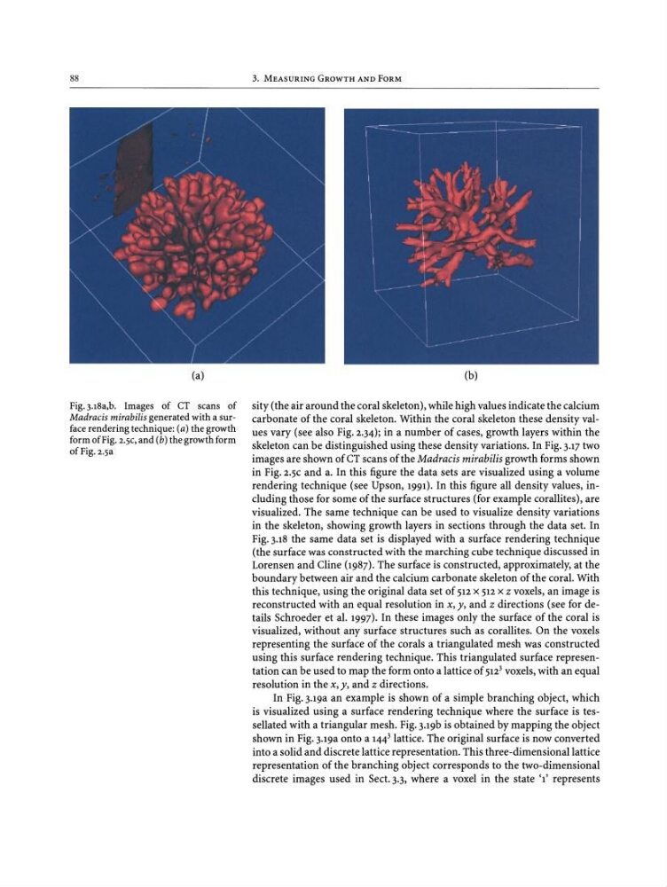
Pig.j.isa.b. Images of CT scans of
Madracis mirabilis generatedwith a surface renderingtechnique: (a) the growth
formofFig. 2.5C, and (b) thegrowthform
of Fig. 2.5a
(b)
sity (the air around the coral skeleton), while high values indicate the calcium
carbonate of the coral skeleton. Within the coral skeleton these density values vary (see also Fig. 2.34); in a number of cases, growth layers within the
skeleton can be distinguished using these density variations. In Fig.3.17 two
images are shown of CT scans of the Madracis mirabilis growth forms shown
in Fig. 2.5C and a. In this figure the data sets are visualized using a volume
rendering technique (see Upson, 1991). In this figure all density values, including those for some of the surface structures (for example corallites), are
visualized. The same technique can be used to visualize density variations
in the skeleton, showing growth layers in sections through the data set. In
Fig. J.i8 the same data set is displayed with a surface rendering technique
(the surface was constructed with the marching cube technique discussed in
Lorensen and Cline (1987). The surface is constructed, approximately, at the
boundary between air and the calcium carbonate skeleton of the coral. With
this technique, using the original data set of 512 x 512 X z voxels, an image is
reconstructed with an equal resolution in x, y, and z directions (see for details Schroeder et al. 1997). In these images only the surface of the coral is
visualized, without any surface structures such as corallites . On the voxels
representing the surface of the corals a triangulated mesh was constructed
using this surface rendering technique. This triangulated surface representation can be used to map the form onto a lattice of 512 3 voxels, with an equal
resolution in the x, y, and z directions.
In Fig.3.19a an example is shown of a simple branching object, which
is visualized using a surface rendering technique where the surface is tessellated with a triangular mesh. Fig. 3.19b is obtained by mapping the object
shown in Fig. J.i9a onto a 144
3 lattice . The original surface is now converted
into a solid and discrete lattice representation. This three-dimensional lattice
representation of the branching object corresponds to the two-dimensional
discrete images used in Sect. 3.3, where a voxel in the state '1' represents
3. MEASURING GROWTH AND FORM
(a)
Pig.j.isa.b. Images of CT scans of
Madracis mirabilis generatedwith a surface renderingtechnique: (a) the growth
formofFig. 2.5C, and (b) thegrowthform
of Fig. 2.5a
(b)
sity (the air around the coral skeleton), while high values indicate the calcium
carbonate of the coral skeleton. Within the coral skeleton these density values vary (see also Fig. 2.34); in a number of cases, growth layers within the
skeleton can be distinguished using these density variations. In Fig.3.17 two
images are shown of CT scans of the Madracis mirabilis growth forms shown
in Fig. 2.5C and a. In this figure the data sets are visualized using a volume
rendering technique (see Upson, 1991). In this figure all density values, including those for some of the surface structures (for example corallites), are
visualized. The same technique can be used to visualize density variations
in the skeleton, showing growth layers in sections through the data set. In
Fig. J.i8 the same data set is displayed with a surface rendering technique
(the surface was constructed with the marching cube technique discussed in
Lorensen and Cline (1987). The surface is constructed, approximately, at the
boundary between air and the calcium carbonate skeleton of the coral. With
this technique, using the original data set of 512 x 512 X z voxels, an image is
reconstructed with an equal resolution in x, y, and z directions (see for details Schroeder et al. 1997). In these images only the surface of the coral is
visualized, without any surface structures such as corallites . On the voxels
representing the surface of the corals a triangulated mesh was constructed
using this surface rendering technique. This triangulated surface representation can be used to map the form onto a lattice of 512 3 voxels, with an equal
resolution in the x, y, and z directions.
In Fig.3.19a an example is shown of a simple branching object, which
is visualized using a surface rendering technique where the surface is tessellated with a triangular mesh. Fig. 3.19b is obtained by mapping the object
shown in Fig. J.i9a onto a 144
3 lattice . The original surface is now converted
into a solid and discrete lattice representation. This three-dimensional lattice
representation of the branching object corresponds to the two-dimensional
discrete images used in Sect. 3.3, where a voxel in the state '1' represents