

if these values are known, the general solution is:
u z
ð Þ ¼
g
rN z
r x
z
3
6
þ
h
2
z
2
À
h
3
3
þ
1
2
Â
g
N z
Z x z
2
À h
2
À
Á þ
t W
rN z
z À h
ð
Þ ð27Þ
or in nondimensional depth Z ¼
z
h
j j ,
u Z
ð Þ ¼
g
6N z r
r x h
3 Z
3
þ 3Z
2
À 2
À
Á þ
1
2
Â
g
N z
Z x h
2 Z
2
À 1
À
Á þ
t W h
rN z
Z þ 1
ð
Þ ð28Þ
This solution is still dependent on the second unknown
(Z x ) and we must apply the integral boundary condition,
written in terms of the nondimensional depth Z:
Z 0
À1
u Z
ð ÞdZ ¼
Q f
A
¼ u f ;
ð29Þ
and the result for the surface slope Z x is:
Z x ¼ À
3N z
gh
2
u f À
15
24
r x
r
h þ 3
t W
rgh
ð30Þ
and depends on three quantities: (1) the fresh water velocity, (2) the baroclinic component and (3) the wind stress.
An order of magnitude analysis indicates that the
baroclinic term, associated with the longitudinal density
gradient, is the dominant equivalent to the M. Margules
rule for the slope of an interface in the atmosphere, which
was adapted to oceanographic use by A. Defant in 1929
(quoted in von Arx, 1962, 383).
Combining (28) and (30), the final solution for u ¼ u
(Z) is Officer (1976):
u Z
ð Þ ¼
gh
3
48N z r
r x 8Z
3
þ 9Z
2
À 1
À
Á
þ
3
2
u f Z
2
À 1
À
Á þ
1
4
Â
h
rN z
t W À3Z
2
À 4Z À 1
À
Á
ð31Þ
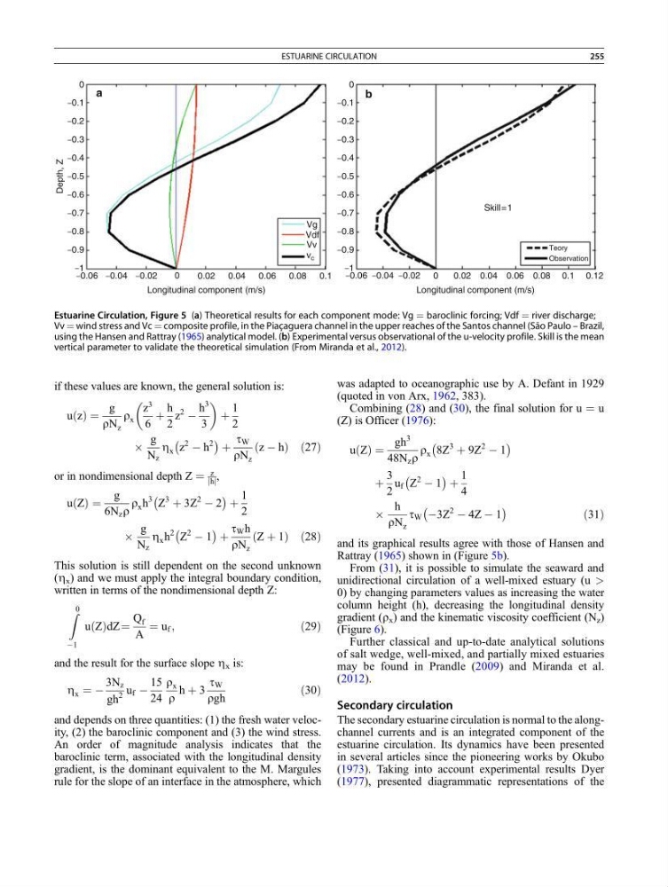
and its graphical results agree with those of Hansen and
Rattray (1965) shown in (Figure 5b).
From (31), it is possible to simulate the seaward and
unidirectional circulation of a well-mixed estuary (u >
0) by changing parameters values as increasing the water
column height (h), decreasing the longitudinal density
gradient (r x ) and the kinematic viscosity coefficient (N z )
(Figure 6).
Further classical and up-to-date analytical solutions
of salt wedge, well-mixed, and partially mixed estuaries
may be found in Prandle (2009) and Miranda et al.
(2012).
Secondary circulation
The secondary estuarine circulation is normal to the alongchannel currents and is an integrated component of the
estuarine circulation. Its dynamics have been presented
in several articles since the pioneering works by Okubo
(1973). Taking into account experimental results Dyer
(1977), presented diagrammatic representations of the
0 a
–0.1
–0.2
–0.3
–0.4
–0.5
–0.6
–0.7
–0.8
–0.9
–1
–0.06 –0.04 –0.02
0.02 0.04 0.06 0.08
Vg
Vdf
Vv
v c
0.1
0
Longitudinal component (m/s)
Longitudinal component (m/s)
0
–0.1
–0.2
–0.3
–0.4
–0.5
–0.6
–0.7
–0.8
–0.9
–1
–0.06 –0.04 –0.02
0.02 0.04 0.06
Skill=1
Teory
Observation
0.08 0.1 0.12
0
Depth, Z
b
Estuarine Circulation, Figure 5 (a) Theoretical results for each component mode: Vg ¼ baroclinic forcing; Vdf ¼ river discharge;
Vv ¼ wind stress and Vc ¼ composite profile, in the Piac ¸aguera channel in the upper reaches of the Santos channel (Sa ˜o Paulo – Brazil,
using the Hansen and Rattray (1965) analytical model. (b) Experimental versus observational of the u-velocity profile. Skill is the mean
vertical parameter to validate the theoretical simulation (From Miranda et al., 2012).
ESTUARINE CIRCULATION
255
u z
ð Þ ¼
g
rN z
r x
z
3
6
þ
h
2
z
2
À
h
3
3
þ
1
2
Â
g
N z
Z x z
2
À h
2
À
Á þ
t W
rN z
z À h
ð
Þ ð27Þ
or in nondimensional depth Z ¼
z
h
j j ,
u Z
ð Þ ¼
g
6N z r
r x h
3 Z
3
þ 3Z
2
À 2
À
Á þ
1
2
Â
g
N z
Z x h
2 Z
2
À 1
À
Á þ
t W h
rN z
Z þ 1
ð
Þ ð28Þ
This solution is still dependent on the second unknown
(Z x ) and we must apply the integral boundary condition,
written in terms of the nondimensional depth Z:
Z 0
À1
u Z
ð ÞdZ ¼
Q f
A
¼ u f ;
ð29Þ
and the result for the surface slope Z x is:
Z x ¼ À
3N z
gh
2
u f À
15
24
r x
r
h þ 3
t W
rgh
ð30Þ
and depends on three quantities: (1) the fresh water velocity, (2) the baroclinic component and (3) the wind stress.
An order of magnitude analysis indicates that the
baroclinic term, associated with the longitudinal density
gradient, is the dominant equivalent to the M. Margules
rule for the slope of an interface in the atmosphere, which
was adapted to oceanographic use by A. Defant in 1929
(quoted in von Arx, 1962, 383).
Combining (28) and (30), the final solution for u ¼ u
(Z) is Officer (1976):
u Z
ð Þ ¼
gh
3
48N z r
r x 8Z
3
þ 9Z
2
À 1
À
Á
þ
3
2
u f Z
2
À 1
À
Á þ
1
4
Â
h
rN z
t W À3Z
2
À 4Z À 1
À
Á
ð31Þ
and its graphical results agree with those of Hansen and
Rattray (1965) shown in (Figure 5b).
From (31), it is possible to simulate the seaward and
unidirectional circulation of a well-mixed estuary (u >
0) by changing parameters values as increasing the water
column height (h), decreasing the longitudinal density
gradient (r x ) and the kinematic viscosity coefficient (N z )
(Figure 6).
Further classical and up-to-date analytical solutions
of salt wedge, well-mixed, and partially mixed estuaries
may be found in Prandle (2009) and Miranda et al.
(2012).
Secondary circulation
The secondary estuarine circulation is normal to the alongchannel currents and is an integrated component of the
estuarine circulation. Its dynamics have been presented
in several articles since the pioneering works by Okubo
(1973). Taking into account experimental results Dyer
(1977), presented diagrammatic representations of the
0 a
–0.1
–0.2
–0.3
–0.4
–0.5
–0.6
–0.7
–0.8
–0.9
–1
–0.06 –0.04 –0.02
0.02 0.04 0.06 0.08
Vg
Vdf
Vv
v c
0.1
0
Longitudinal component (m/s)
Longitudinal component (m/s)
0
–0.1
–0.2
–0.3
–0.4
–0.5
–0.6
–0.7
–0.8
–0.9
–1
–0.06 –0.04 –0.02
0.02 0.04 0.06
Skill=1
Teory
Observation
0.08 0.1 0.12
0
Depth, Z
b
Estuarine Circulation, Figure 5 (a) Theoretical results for each component mode: Vg ¼ baroclinic forcing; Vdf ¼ river discharge;
Vv ¼ wind stress and Vc ¼ composite profile, in the Piac ¸aguera channel in the upper reaches of the Santos channel (Sa ˜o Paulo – Brazil,
using the Hansen and Rattray (1965) analytical model. (b) Experimental versus observational of the u-velocity profile. Skill is the mean
vertical parameter to validate the theoretical simulation (From Miranda et al., 2012).
ESTUARINE CIRCULATION
255