

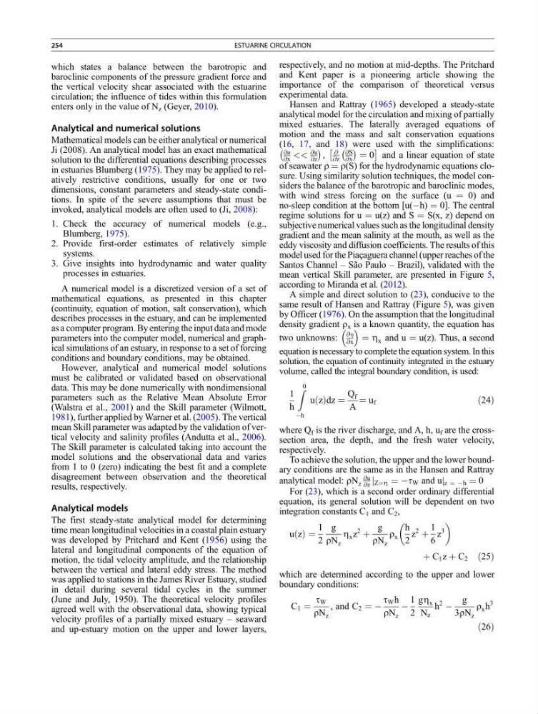
which states a balance between the barotropic and
baroclinic components of the pressure gradient force and
the vertical velocity shear associated with the estuarine
circulation; the influence of tides within this formulation
enters only in the value of N z (Geyer, 2010).
Analytical and numerical solutions
Mathematical models can be either analytical or numerical
Ji (2008). An analytical model has an exact mathematical
solution to the differential equations describing processes
in estuaries Blumberg (1975). They may be applied to relatively restrictive conditions, usually for one or two
dimensions, constant parameters and steady-state conditions. In spite of the severe assumptions that must be
invoked, analytical models are often used to (Ji, 2008):
1. Check the accuracy of numerical models (e.g.,
Blumberg, 1975).
2. Provide first-order estimates of relatively simple
systems.
3. Give insights into hydrodynamic and water quality
processes in estuaries.
A numerical model is a discretized version of a set of
mathematical equations, as presented in this chapter
(continuity, equation of motion, salt conservation), which
describes processes in the estuary, and can be implemented
as a computer program. By entering the input data and mode
parameters into the computer model, numerical and graphical simulations of an estuary, in response to a set of forcing
conditions and boundary conditions, may be obtained.
However, analytical and numerical model solutions
must be calibrated or validated based on observational
data. This may be done numerically with nondimensional
parameters such as the Relative Mean Absolute Error
(Walstra et al., 2001) and the Skill parameter (Wilmott,
1981), further applied by Warner et al. (2005). The vertical
mean Skill parameter was adapted by the validation of vertical velocity and salinity profiles (Andutta et al., 2006).
The Skill parameter is calculated taking into account the
model solutions and the observational data and varies
from 1 to 0 (zero) indicating the best fit and a complete
disagreement between observation and the theoretical
results, respectively.
Analytical models
The first steady-state analytical model for determining
time mean longitudinal velocities in a coastal plain estuary
was developed by Pritchard and Kent (1956) using the
lateral and longitudinal components of the equation of
motion, the tidal velocity amplitude, and the relationship
between the vertical and lateral eddy stress. The method
was applied to stations in the James River Estuary, studied
in detail during several tidal cycles in the summer
(June and July, 1950). The theoretical velocity profiles
agreed well with the observational data, showing typical
velocity profiles of a partially mixed estuary – seaward
and up-estuary motion on the upper and lower layers,
respectively, and no motion at mid-depths. The Pritchard
and Kent paper is a pioneering article showing the
importance of the comparison of theoretical versus
experimental data.
Hansen and Rattray (1965) developed a steady-state
analytical model for the circulation and mixing of partially
mixed estuaries. The laterally averaged equations of
motion and the mass and salt conservation equations
(16, 17, and 18) were used with the simplifications:
@u
@x <<
@u
@z
À
Á
,
@
@z
@S
@x
À Á ¼ 0
Â
Ã
and a linear equation of state
of seawater r ¼ r(S) for the hydrodynamic equations closure. Using similarity solution techniques, the model considers the balance of the barotropic and baroclinic modes,
with wind stress forcing on the surface (u ¼ 0) and
no-sleep condition at the bottom [u(Àh) ¼ 0]. The central
regime solutions for u ¼ u(z) and S ¼ S(x, z) depend on
subjective numerical values such as the longitudinal density
gradient and the mean salinity at the mouth, as well as the
eddy viscosity and diffusion coefficients. The results of this
model used for the Piaçaguera channel (upper reaches of the
Santos Channel – São Paulo – Brazil), validated with the
mean vertical Skill parameter, are presented in Figure 5,
according to Miranda et al. (2012).
A simple and direct solution to (23), conducive to the
same result of Hansen and Rattray (Figure 5), was given
by Officer (1976). On the assumption that the longitudinal
density gradient r x is a known quantity, the equation has
two unknowns:
@
@x
¼ Z x and u ¼ u(z). Thus, a second
equation is necessary to complete the equation system. In this
solution, the equation of continuity integrated in the estuary
volume, called the integral boundary condition, is used:
1
h
Z 0
Àh
u z
ð Þdz ¼
Q f
A
¼ u f
ð24Þ
where Q f is the river discharge, and A, h, u f are the crosssection area, the depth, and the fresh water velocity,
respectively.
To achieve the solution, the upper and the lower boundary conditions are the same as in the Hansen and Rattray
analytical model: rN z
@u
@z j Z¼Z ¼ Àt W and u| z ¼ Àh ¼ 0
For (23), which is a second order ordinary differential
equation, its general solution will be dependent on two
integration constants C 1 and C 2 ,
u z
ð Þ ¼
1
2
g
rN z
Z x z
2
þ
g
rN z
r x
h
2
z
2
þ
1
6
z
3
þ C 1 z þ C 2 ð25Þ
which are determined according to the upper and lower
boundary conditions:
C 1 ¼
t W
rN z
, and C 2 ¼ À
t W h
rN z
À
1
2
gZ x
N z
h
2
À
g
3rN z
r x h
3
ð26Þ
254
ESTUARINE CIRCULATION
baroclinic components of the pressure gradient force and
the vertical velocity shear associated with the estuarine
circulation; the influence of tides within this formulation
enters only in the value of N z (Geyer, 2010).
Analytical and numerical solutions
Mathematical models can be either analytical or numerical
Ji (2008). An analytical model has an exact mathematical
solution to the differential equations describing processes
in estuaries Blumberg (1975). They may be applied to relatively restrictive conditions, usually for one or two
dimensions, constant parameters and steady-state conditions. In spite of the severe assumptions that must be
invoked, analytical models are often used to (Ji, 2008):
1. Check the accuracy of numerical models (e.g.,
Blumberg, 1975).
2. Provide first-order estimates of relatively simple
systems.
3. Give insights into hydrodynamic and water quality
processes in estuaries.
A numerical model is a discretized version of a set of
mathematical equations, as presented in this chapter
(continuity, equation of motion, salt conservation), which
describes processes in the estuary, and can be implemented
as a computer program. By entering the input data and mode
parameters into the computer model, numerical and graphical simulations of an estuary, in response to a set of forcing
conditions and boundary conditions, may be obtained.
However, analytical and numerical model solutions
must be calibrated or validated based on observational
data. This may be done numerically with nondimensional
parameters such as the Relative Mean Absolute Error
(Walstra et al., 2001) and the Skill parameter (Wilmott,
1981), further applied by Warner et al. (2005). The vertical
mean Skill parameter was adapted by the validation of vertical velocity and salinity profiles (Andutta et al., 2006).
The Skill parameter is calculated taking into account the
model solutions and the observational data and varies
from 1 to 0 (zero) indicating the best fit and a complete
disagreement between observation and the theoretical
results, respectively.
Analytical models
The first steady-state analytical model for determining
time mean longitudinal velocities in a coastal plain estuary
was developed by Pritchard and Kent (1956) using the
lateral and longitudinal components of the equation of
motion, the tidal velocity amplitude, and the relationship
between the vertical and lateral eddy stress. The method
was applied to stations in the James River Estuary, studied
in detail during several tidal cycles in the summer
(June and July, 1950). The theoretical velocity profiles
agreed well with the observational data, showing typical
velocity profiles of a partially mixed estuary – seaward
and up-estuary motion on the upper and lower layers,
respectively, and no motion at mid-depths. The Pritchard
and Kent paper is a pioneering article showing the
importance of the comparison of theoretical versus
experimental data.
Hansen and Rattray (1965) developed a steady-state
analytical model for the circulation and mixing of partially
mixed estuaries. The laterally averaged equations of
motion and the mass and salt conservation equations
(16, 17, and 18) were used with the simplifications:
@u
@x <<
@u
@z
À
Á
,
@
@z
@S
@x
À Á ¼ 0
Â
Ã
and a linear equation of state
of seawater r ¼ r(S) for the hydrodynamic equations closure. Using similarity solution techniques, the model considers the balance of the barotropic and baroclinic modes,
with wind stress forcing on the surface (u ¼ 0) and
no-sleep condition at the bottom [u(Àh) ¼ 0]. The central
regime solutions for u ¼ u(z) and S ¼ S(x, z) depend on
subjective numerical values such as the longitudinal density
gradient and the mean salinity at the mouth, as well as the
eddy viscosity and diffusion coefficients. The results of this
model used for the Piaçaguera channel (upper reaches of the
Santos Channel – São Paulo – Brazil), validated with the
mean vertical Skill parameter, are presented in Figure 5,
according to Miranda et al. (2012).
A simple and direct solution to (23), conducive to the
same result of Hansen and Rattray (Figure 5), was given
by Officer (1976). On the assumption that the longitudinal
density gradient r x is a known quantity, the equation has
two unknowns:
@
@x
¼ Z x and u ¼ u(z). Thus, a second
equation is necessary to complete the equation system. In this
solution, the equation of continuity integrated in the estuary
volume, called the integral boundary condition, is used:
1
h
Z 0
Àh
u z
ð Þdz ¼
Q f
A
¼ u f
ð24Þ
where Q f is the river discharge, and A, h, u f are the crosssection area, the depth, and the fresh water velocity,
respectively.
To achieve the solution, the upper and the lower boundary conditions are the same as in the Hansen and Rattray
analytical model: rN z
@u
@z j Z¼Z ¼ Àt W and u| z ¼ Àh ¼ 0
For (23), which is a second order ordinary differential
equation, its general solution will be dependent on two
integration constants C 1 and C 2 ,
u z
ð Þ ¼
1
2
g
rN z
Z x z
2
þ
g
rN z
r x
h
2
z
2
þ
1
6
z
3
þ C 1 z þ C 2 ð25Þ
which are determined according to the upper and lower
boundary conditions:
C 1 ¼
t W
rN z
, and C 2 ¼ À
t W h
rN z
À
1
2
gZ x
N z
h
2
À
g
3rN z
r x h
3
ð26Þ
254
ESTUARINE CIRCULATION