

a depth z up to the sea surface slope Z(x, y, t) (relative to
a level surface):
p x, y, z, t
ð
Þ¼p a x, y, t
ð
Þþg
Z Z
z
rdz
ð19Þ
where p a is the atmospheric pressure on the sea surface.
Taking the differential of (19) using the Leibnitz differentiation rule it follows that:
@p
@x
¼
@p a
@x
þ g r Z
@Z
@x
þ
Z Z
z
@r
@x
dz
0
@
1
A
2
4
3
5
ð20Þ
where r Z is the density on the surface. From this result,
with
r Z
r % 1, the expression for the longitudinal component
of the gradient pressure force (per mass unit) has three
components:
À
1
r
@p
@x
¼ À
1
r
@p a
@x
À g
@Z
@x
À
g
r
Z Z
z
@r
@x
dz
ð21Þ
namely, barometric (a), barotropic (b), and baroclinic (c),
respectively:
(a) The barometric component is related to transient
weather systems (typically 3–10 days) associated with
low-pressure centers and has subtidal variability.
Under steady state, the sea surface acts as an inverted
barometer; for Dp ¼ Æ1.0 mbar the sea surface
decreases/increases by 1.0 cm. However, if a storm
surge was to reach an estuary, it may cause severe dangerous floods, especially during spring tide.
(b) Is independent of depth and varies according to the
sea surface slope oscillation. In normal tidal
conditions, its highest and smallest values occur during the spring and neap tide, respectively. Its order
of magnitude varies approximately in the interval
À10
À3
– +10
À3 (ms
À2
). Thus, it is considered to
have inter or subtidal variability.
(c) This component is zero on the surface (z ¼ Z) and
increases with the depth, up to a magnitude order of
À10
À4 ms
À2
. Due to the inter and subtidal variability
of the density field, its numerical value is not an easy
quantity to be determined.
During the flood tides, barotropic (b) and baroclinic
(c) forces act up-estuary, but during the ebb they act in
the opposite direction.
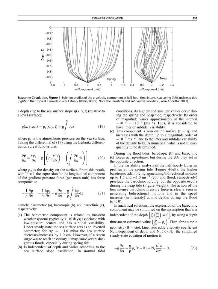
In the variability analysis of the half-hourly Eulerian
profiles at the spring tide (Figure 4-left), the higher
barotropic tidal forcing, generating bidirectional motions
up to 1.5 and À1.0 ms
À1 (ebb and flood, respectively)
preclude the baroclinic forcing, but the opposite occurs
during the neap tide (Figure 4-right). The action of the
less intense baroclinic pressure force is clearly seen in
generating bidirectional motions and in the speed
increase (in intensity) at mid-depths during the flood
(u < 0).
In analytical solutions, the expression of the baroclinic
component may be simplified on the assumption that it is
independent of the depth
@
@z
@r
@x
¼ 0
h
i
, by using a depth
time-mean estimated value
@r
@x ¼ r x
. Then, for a simple
geometry (B ¼ cte), kinematic eddy viscosity coefficient
N z independent of depth and N z >> N x , the simplified
steady-state equation of motion is:
Àg
@Z
@x
À
g
r
r x z þ h
ð
ÞþN z
@
2 u
@z 2 ¼ 0;
ð23Þ
0
–0.1
–0.2
–0.3
–0.4
–0.5
–0.6
–0.7
–0.8
–0.9
–1
–1.5
–1
–0.5
–0.4
–0.2
0
0.2
0.4
Neap
Spring
u-Component (m/s)
u–Component (m/s)
0.5
1
1.5
0
Depth, Z
Estuarine Circulation, Figure 4 Eulerian profiles of the u-velocity component at half-hour time intervals at spring (left) and neap tide
(right) in the tropical Caravelas River Estuary (Bahia, Brazil). Note the intratidal and subtidal variabilities (From Andutta, 2011).
ESTUARINE CIRCULATION
253
a level surface):
p x, y, z, t
ð
Þ¼p a x, y, t
ð
Þþg
Z Z
z
rdz
ð19Þ
where p a is the atmospheric pressure on the sea surface.
Taking the differential of (19) using the Leibnitz differentiation rule it follows that:
@p
@x
¼
@p a
@x
þ g r Z
@Z
@x
þ
Z Z
z
@r
@x
dz
0
@
1
A
2
4
3
5
ð20Þ
where r Z is the density on the surface. From this result,
with
r Z
r % 1, the expression for the longitudinal component
of the gradient pressure force (per mass unit) has three
components:
À
1
r
@p
@x
¼ À
1
r
@p a
@x
À g
@Z
@x
À
g
r
Z Z
z
@r
@x
dz
ð21Þ
namely, barometric (a), barotropic (b), and baroclinic (c),
respectively:
(a) The barometric component is related to transient
weather systems (typically 3–10 days) associated with
low-pressure centers and has subtidal variability.
Under steady state, the sea surface acts as an inverted
barometer; for Dp ¼ Æ1.0 mbar the sea surface
decreases/increases by 1.0 cm. However, if a storm
surge was to reach an estuary, it may cause severe dangerous floods, especially during spring tide.
(b) Is independent of depth and varies according to the
sea surface slope oscillation. In normal tidal
conditions, its highest and smallest values occur during the spring and neap tide, respectively. Its order
of magnitude varies approximately in the interval
À10
À3
– +10
À3 (ms
À2
). Thus, it is considered to
have inter or subtidal variability.
(c) This component is zero on the surface (z ¼ Z) and
increases with the depth, up to a magnitude order of
À10
À4 ms
À2
. Due to the inter and subtidal variability
of the density field, its numerical value is not an easy
quantity to be determined.
During the flood tides, barotropic (b) and baroclinic
(c) forces act up-estuary, but during the ebb they act in
the opposite direction.
In the variability analysis of the half-hourly Eulerian
profiles at the spring tide (Figure 4-left), the higher
barotropic tidal forcing, generating bidirectional motions
up to 1.5 and À1.0 ms
À1 (ebb and flood, respectively)
preclude the baroclinic forcing, but the opposite occurs
during the neap tide (Figure 4-right). The action of the
less intense baroclinic pressure force is clearly seen in
generating bidirectional motions and in the speed
increase (in intensity) at mid-depths during the flood
(u < 0).
In analytical solutions, the expression of the baroclinic
component may be simplified on the assumption that it is
independent of the depth
@
@z
@r
@x
¼ 0
h
i
, by using a depth
time-mean estimated value
@r
@x ¼ r x
. Then, for a simple
geometry (B ¼ cte), kinematic eddy viscosity coefficient
N z independent of depth and N z >> N x , the simplified
steady-state equation of motion is:
Àg
@Z
@x
À
g
r
r x z þ h
ð
ÞþN z
@
2 u
@z 2 ¼ 0;
ð23Þ
0
–0.1
–0.2
–0.3
–0.4
–0.5
–0.6
–0.7
–0.8
–0.9
–1
–1.5
–1
–0.5
–0.4
–0.2
0
0.2
0.4
Neap
Spring
u-Component (m/s)
u–Component (m/s)
0.5
1
1.5
0
Depth, Z
Estuarine Circulation, Figure 4 Eulerian profiles of the u-velocity component at half-hour time intervals at spring (left) and neap tide
(right) in the tropical Caravelas River Estuary (Bahia, Brazil). Note the intratidal and subtidal variabilities (From Andutta, 2011).
ESTUARINE CIRCULATION
253