

the symbol < > indicates “time mean value” of the correlations of small-scale velocity components multiplied by
the small-scale salinity variation. These values, multiplied
by the density (K x ¼ À r < u
0 S
0
>; K y ¼ À r < v
0 S
0
>;
K z ¼ À r < w
0 S
0
>), are the salt fluxes [ML
À2
T
À1
] generated by turbulent diffusion.
The equations of motion are based on Newton’s second
law applied to the fluids, taking into account the forces and
energy dissipation. The equation for a turbulent fluid was
also presented in the classic paper of O. Reynolds. However, the estuarine water body has a particular geometry
and has one open surface boundary; thus, special attention
will be paid to the simplifications for their analytical and
numerical solutions. For a hydrostatic fluid the equations
of motion are:
@u
@t
þ u
@u
@x
þ v
@u
@y
w
@u
@z
À fv
¼ À
1
r
@p
@x
þ
@
@x
N x
@u
@x
þ
@
@y
N y
@u
@y
þ
@
@z
N z
@u
@z
ð13Þ
@v
@t
þ u
@v
@x
þ v
@v
@y
w
@v
@z
þ fu
¼ À
1
r
@p
@y
þ
@
@x
N x
@v
@x
þ
@
@y
N y
@v
@y
þ
@
@z
N z
@v
@z
ð14Þ
1
r
@p
@z
¼ Àg
ð15Þ
where f is the Coriolis parameter [f ¼ 2 Â Osin(y), O
is the angular velocity of the earth and y is the latitude],
and g is the acceleration of gravity. In (11) and (14) N x
(K x ), N y (K y ), and N z (K z ) are the eddy kinematic viscosity (diffusion) coefficients. Since the estuarine water
mass is assumed to be a system composed of pure
water + salt, it will also be necessary to include in
the hydrodynamic framework the equation of state of
seawater, and the mass and salt conservation equations
(4 and 11).
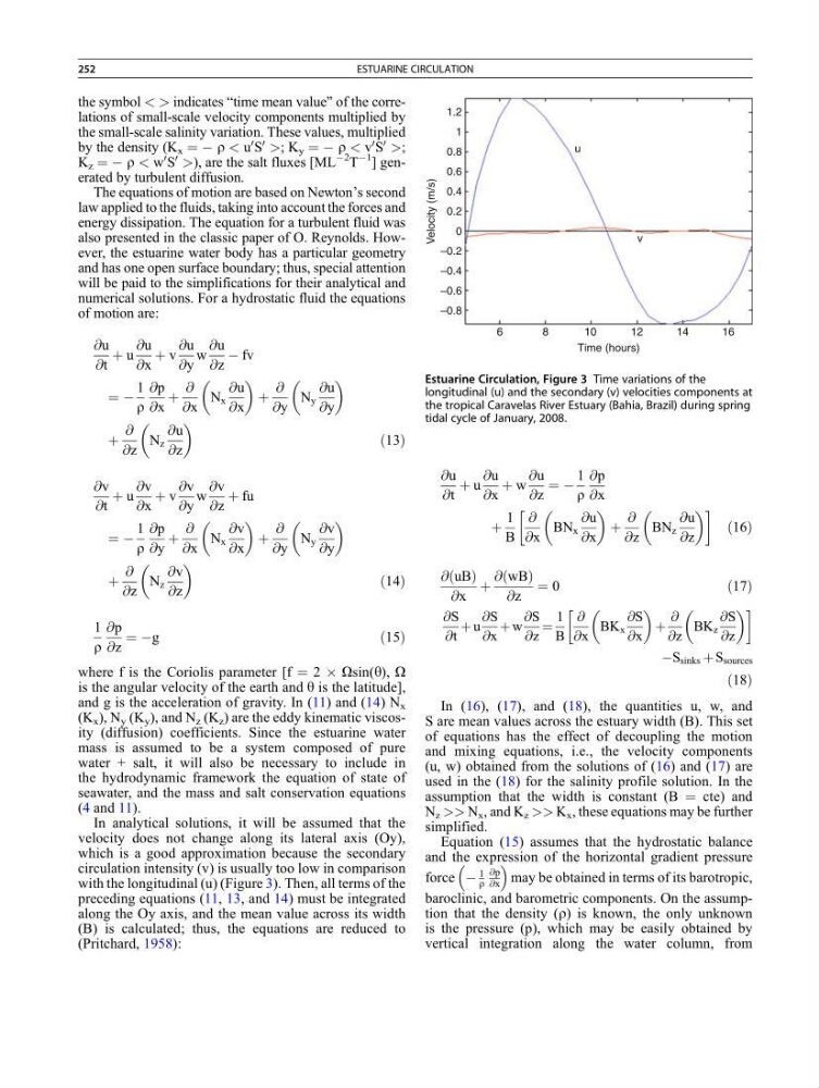
In analytical solutions, it will be assumed that the
velocity does not change along its lateral axis (Oy),
which is a good approximation because the secondary
circulation intensity (v) is usually too low in comparison
with the longitudinal (u) (Figure 3). Then, all terms of the
preceding equations (11, 13, and 14) must be integrated
along the Oy axis, and the mean value across its width
(B) is calculated; thus, the equations are reduced to
(Pritchard, 1958):
@u
@t
þ u
@u
@x
þ w
@u
@z
¼ À
1
r
@p
@x
þ
1
B
@
@x
BN x
@u
@x
þ
@
@z
BN z
@u
@z
!
ð16Þ
@ uB
ð Þ
@x
þ
@ wB
ð Þ
@z
¼ 0
ð17Þ
@S
@t
þ u
@S
@x
þ w
@S
@z
¼
1
B
@
@x
BK x
@S
@x
þ
@
@z
BK z
@S
@z
!
ÀS sinks þ S sources
ð18Þ
In (16), (17), and (18), the quantities u, w, and
S are mean values across the estuary width (B). This set
of equations has the effect of decoupling the motion
and mixing equations, i.e., the velocity components
(u, w) obtained from the solutions of (16) and (17) are
used in the (18) for the salinity profile solution. In the
assumption that the width is constant (B ¼ cte) and
N z >> N x , and K z >> K x , these equations may be further
simplified.
Equation (15) assumes that the hydrostatic balance
and the expression of the horizontal gradient pressure
force À
1
r
@p
@x
may be obtained in terms of its barotropic,
baroclinic, and barometric components. On the assumption that the density (r) is known, the only unknown
is the pressure (p), which may be easily obtained by
vertical integration along the water column, from
1.2
1
0.8
u
v
0.6
0.4
0.2
Velocity (m/s)
0
–0.2
–0.4
–0.6
–0.8
6
8
1 0
Time (hours)
12
14
16
Estuarine Circulation, Figure 3 Time variations of the
longitudinal (u) and the secondary (v) velocities components at
the tropical Caravelas River Estuary (Bahia, Brazil) during spring
tidal cycle of January, 2008.
252
ESTUARINE CIRCULATION
the small-scale salinity variation. These values, multiplied
by the density (K x ¼ À r < u
0 S
0
>; K y ¼ À r < v
0 S
0
>;
K z ¼ À r < w
0 S
0
>), are the salt fluxes [ML
À2
T
À1
] generated by turbulent diffusion.
The equations of motion are based on Newton’s second
law applied to the fluids, taking into account the forces and
energy dissipation. The equation for a turbulent fluid was
also presented in the classic paper of O. Reynolds. However, the estuarine water body has a particular geometry
and has one open surface boundary; thus, special attention
will be paid to the simplifications for their analytical and
numerical solutions. For a hydrostatic fluid the equations
of motion are:
@u
@t
þ u
@u
@x
þ v
@u
@y
w
@u
@z
À fv
¼ À
1
r
@p
@x
þ
@
@x
N x
@u
@x
þ
@
@y
N y
@u
@y
þ
@
@z
N z
@u
@z
ð13Þ
@v
@t
þ u
@v
@x
þ v
@v
@y
w
@v
@z
þ fu
¼ À
1
r
@p
@y
þ
@
@x
N x
@v
@x
þ
@
@y
N y
@v
@y
þ
@
@z
N z
@v
@z
ð14Þ
1
r
@p
@z
¼ Àg
ð15Þ
where f is the Coriolis parameter [f ¼ 2 Â Osin(y), O
is the angular velocity of the earth and y is the latitude],
and g is the acceleration of gravity. In (11) and (14) N x
(K x ), N y (K y ), and N z (K z ) are the eddy kinematic viscosity (diffusion) coefficients. Since the estuarine water
mass is assumed to be a system composed of pure
water + salt, it will also be necessary to include in
the hydrodynamic framework the equation of state of
seawater, and the mass and salt conservation equations
(4 and 11).
In analytical solutions, it will be assumed that the
velocity does not change along its lateral axis (Oy),
which is a good approximation because the secondary
circulation intensity (v) is usually too low in comparison
with the longitudinal (u) (Figure 3). Then, all terms of the
preceding equations (11, 13, and 14) must be integrated
along the Oy axis, and the mean value across its width
(B) is calculated; thus, the equations are reduced to
(Pritchard, 1958):
@u
@t
þ u
@u
@x
þ w
@u
@z
¼ À
1
r
@p
@x
þ
1
B
@
@x
BN x
@u
@x
þ
@
@z
BN z
@u
@z
!
ð16Þ
@ uB
ð Þ
@x
þ
@ wB
ð Þ
@z
¼ 0
ð17Þ
@S
@t
þ u
@S
@x
þ w
@S
@z
¼
1
B
@
@x
BK x
@S
@x
þ
@
@z
BK z
@S
@z
!
ÀS sinks þ S sources
ð18Þ
In (16), (17), and (18), the quantities u, w, and
S are mean values across the estuary width (B). This set
of equations has the effect of decoupling the motion
and mixing equations, i.e., the velocity components
(u, w) obtained from the solutions of (16) and (17) are
used in the (18) for the salinity profile solution. In the
assumption that the width is constant (B ¼ cte) and
N z >> N x , and K z >> K x , these equations may be further
simplified.
Equation (15) assumes that the hydrostatic balance
and the expression of the horizontal gradient pressure
force À
1
r
@p
@x
may be obtained in terms of its barotropic,
baroclinic, and barometric components. On the assumption that the density (r) is known, the only unknown
is the pressure (p), which may be easily obtained by
vertical integration along the water column, from
1.2
1
0.8
u
v
0.6
0.4
0.2
Velocity (m/s)
0
–0.2
–0.4
–0.6
–0.8
6
8
1 0
Time (hours)
12
14
16
Estuarine Circulation, Figure 3 Time variations of the
longitudinal (u) and the secondary (v) velocities components at
the tropical Caravelas River Estuary (Bahia, Brazil) during spring
tidal cycle of January, 2008.
252
ESTUARINE CIRCULATION