

722
21.4.2 Were the Pattern and Amount of Sedimentation
as Expected?
To measure the rate and amount of sediment deposition in the restoration cells, 50
plots with a marker horizon were installed (Fig. 21.5) in early October 2010 (before
the breaching of the old dike). An additional seven marker horizons were installed
in the East reference marsh (Fig. 21.5). The method used was similar to that
described in Bowron et al. (2009). Briefly, each plot was 0.75 m × 0.75 m in size and
a 5 cm × 5 cm wooden post was used to mark it (Fig. 21.11a). The vegetation was
trimmed where necessary and a layer of feldspar clay deposited on the surface
(about 5 mm thick). The location of each plot was measured with Real-Time
Kinematic and Differential GPS (RTK DGPS; Leica 1200 with three-dimensional
accuracy of 2 cm or less). Each subsequent October, the marker horizons were sampled (if possible) using cryogenic coring (Fig. 21.11b, c). A plot was typically relocated using RTK DGPS, since many of the posts installed in 2010 were damaged
(Fig. 21.11b), missing, or buried within the first year. If a marker horizon could not
be located after three cores, it was deemed missing or compromised (eroded). Total
accretion since the marker horizon was installed was estimated by measuring the
amount of material above it (Fig. 21.11c). By measuring at regular temporal
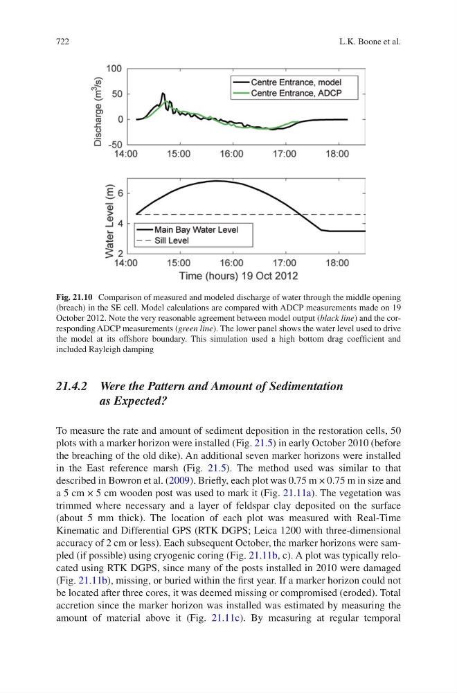
Fig. 21.10 Comparison of measured and modeled discharge of water through the middle opening
(breach) in the SE cell. Model calculations are compared with ADCP measurements made on 19
October 2012. Note the very reasonable agreement between model output (black line) and the corresponding ADCP measurements (green line). The lower panel shows the water level used to drive
the model at its offshore boundary. This simulation used a high bottom drag coefficient and
included Rayleigh damping
L.K. Boone et al.