

721
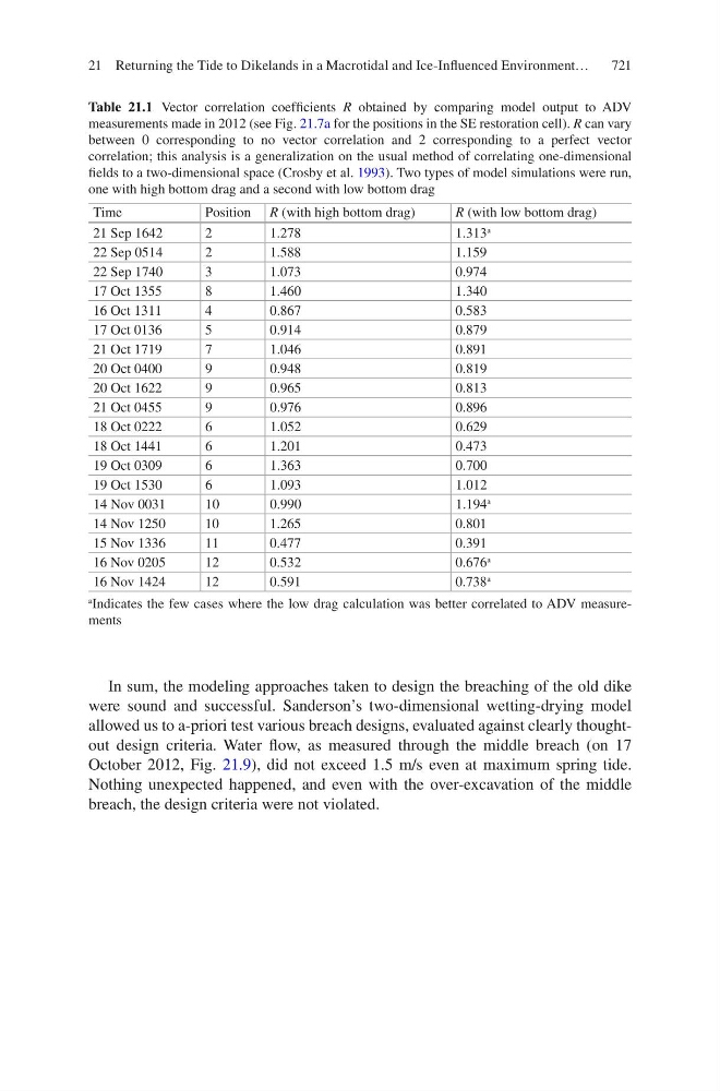
Table 21.1 Vector correlation coefficients R obtained by comparing model output to ADV
measurements made in 2012 (see Fig. 21.7a for the positions in the SE restoration cell). R can vary
between 0 corresponding to no vector correlation and 2 corresponding to a perfect vector
correlation; this analysis is a generalization on the usual method of correlating one-dimensional
fields to a two-dimensional space (Crosby et al. 1993). Two types of model simulations were run,
one with high bottom drag and a second with low bottom drag
Time
Position R (with high bottom drag)
R (with low bottom drag)
21 Sep 1642
2
1.278
1.313
a
22 Sep 0514
2
1.588
1.159
22 Sep 1740
3
1.073
0.974
17 Oct 1355
8
1.460
1.340
16 Oct 1311
4
0.867
0.583
17 Oct 0136
5
0.914
0.879
21 Oct 1719
7
1.046
0.891
20 Oct 0400
9
0.948
0.819
20 Oct 1622
9
0.965
0.813
21 Oct 0455
9
0.976
0.896
18 Oct 0222
6
1.052
0.629
18 Oct 1441
6
1.201
0.473
19 Oct 0309
6
1.363
0.700
19 Oct 1530
6
1.093
1.012
14 Nov 0031
10
0.990
1.194
a
14 Nov 1250
10
1.265
0.801
15 Nov 1336
11
0.477
0.391
16 Nov 0205
12
0.532
0.676
a
16 Nov 1424
12
0.591
0.738
a
a
Indicates the few cases where the low drag calculation was better correlated to ADV measurements
In sum, the modeling approaches taken to design the breaching of the old dike
were sound and successful. Sanderson’s two-dimensional wetting-drying model
allowed us to a-priori test various breach designs, evaluated against clearly thoughtout design criteria. Water flow, as measured through the middle breach (on 17
October 2012, Fig. 21.9), did not exceed 1.5 m/s even at maximum spring tide.
Nothing unexpected happened, and even with the over-excavation of the middle
breach, the design criteria were not violated.
21 Returning the Tide to Dikelands in a Macrotidal and Ice-Influenced Environment…