

24
J.L. Giraudel . S. Lek
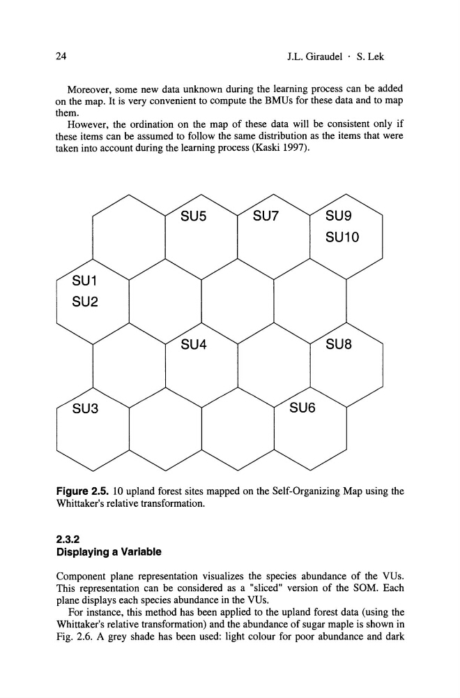
Moreover, some new data unknown during the learning process can be added
on the map. It is very convenient to compute the BMUs for these data and to map
them.
However, the ordination on the map of these data will be consistent only if
these items can be assumed to follow the same distribution as the items that were
taken into account during the learning process (Kaski 1997).
SU1
SU2
SU7
SU6
SU9
SU10
SU8
Figure 2.5. 10 upland forest sites mapped on the Self-Organizing Map using the
Whittaker's relative transformation.
2.3.2
Displaying a Variable
Component plane representation visualizes the species abundance of the VUs.
This representation can be considered as a "sliced" version of the SOM. Each
plane displays each species abundance in the VUs.
For instance, this method has been applied to the upland forest data (using the
Whittaker's relative transformation) and the abundance of sugar maple is shown in
Fig. 2.6. A grey shade has been used: light colour for poor abundance and dark
J.L. Giraudel . S. Lek
Moreover, some new data unknown during the learning process can be added
on the map. It is very convenient to compute the BMUs for these data and to map
them.
However, the ordination on the map of these data will be consistent only if
these items can be assumed to follow the same distribution as the items that were
taken into account during the learning process (Kaski 1997).
SU1
SU2
SU7
SU6
SU9
SU10
SU8
Figure 2.5. 10 upland forest sites mapped on the Self-Organizing Map using the
Whittaker's relative transformation.
2.3.2
Displaying a Variable
Component plane representation visualizes the species abundance of the VUs.
This representation can be considered as a "sliced" version of the SOM. Each
plane displays each species abundance in the VUs.
For instance, this method has been applied to the upland forest data (using the
Whittaker's relative transformation) and the abundance of sugar maple is shown in
Fig. 2.6. A grey shade has been used: light colour for poor abundance and dark