

Chapter 2 . Unsupervised Artificial Neural Networks
23
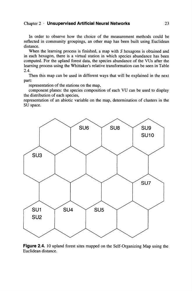
In order to observe how the choice of the measurement methods could be
reflected in community groupings, an other map has been built using Euclidean
distance.
When the learning process is finished, a map with S hexagons is obtained and
in each hexagon, there is a virtual station in which species abundance has been
computed. For the upland forest data, the species abundance of the VUs after the
learning process using the Whittaker's relative transformation can be seen in Table
2.4.
Then this map can be used in different ways that will be explained in the next
part:
representation of the stations on the map,
component planes: the species composition of each VU can be used to display
the distribution of each species,
representation of an abiotic variable on the map, determination of clusters in the
SU space.
SU3
SU1
SU2
SU6
SU4
SU8
SU9
SU10
SU7
Figure 2.4. 10 upland forest sites mapped on the Self-Organizing Map using the
Euclidean distance.
23
In order to observe how the choice of the measurement methods could be
reflected in community groupings, an other map has been built using Euclidean
distance.
When the learning process is finished, a map with S hexagons is obtained and
in each hexagon, there is a virtual station in which species abundance has been
computed. For the upland forest data, the species abundance of the VUs after the
learning process using the Whittaker's relative transformation can be seen in Table
2.4.
Then this map can be used in different ways that will be explained in the next
part:
representation of the stations on the map,
component planes: the species composition of each VU can be used to display
the distribution of each species,
representation of an abiotic variable on the map, determination of clusters in the
SU space.
SU3
SU1
SU2
SU6
SU4
SU8
SU9
SU10
SU7
Figure 2.4. 10 upland forest sites mapped on the Self-Organizing Map using the
Euclidean distance.