

Chapter 2 . Unsupervised Artificial Neural Networks
21
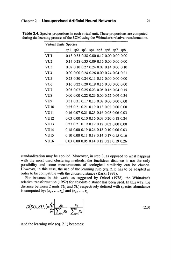
Table 2.4. Species proportions in each virtual unit. These proportions are computed
during the learning process of the SOM using the Whittaker's relative transformation.
Virtual Units Species
VUl
VU2
VU3
VU4
VU5
VU6
VU7
VU8
VU9
VUIO
VUll
VU12
VU13
VU14
VU15
VU16
spl sp2 sp3 sp4 sp5 sp6 sp7 sp8
0.13 0.33 0.38 0.00 0.17 0.00 0.00 0.00
0.14 0.28 0.33 0.09 0.16 0.000.00 0.00
0.070.10 0.270.240.070.140.000.10
0.000.000.240.260.000.240.040.21
0.23 0.300.24 0.11 0.12 0.00 0.00 0.00
0.16 0.22 0.28 0.19 0.16 0.00 0.00 0.00
0.05 0.07 0.25 0.23 0.05 0.16 0.04 0.15
0.00 0.00 0.22 0.23 0.00 0.22 0.09 0.24
0.31 0.31 0.17 0.13 0.07 0.00 0.00 0.00
0.25 0.21 0.21 0.19 0.13 0.02 0.00 0.00
0.16 0.07 0.21 0.23 0.16 0.08 0.06 0.03
0.03 0.000.10 0.16 0.09 0.200.18 0.24
0.27 0.21 0.19 0.19 0.12 0.02 0.00 0.00
0.18 0.00 0.19 0.26 0.18 0.10 0.06 0.03
0.10 0.00 0.11 0.19 0.14 0.17 0.15 0.16
0.03 0.000.05 0.140.12 0.21 0.19 0.26
standardization may be applied. Moreover, in step 3, as opposed to what happens
with the most used clustering methods. the Euclidean distance is not the only
possibility and some measurements of ecological similarity can be chosen.
However, in this case, the use of the learning rule (eq. 2.1) has to be adapted in
order to be compatible with the chosen distance (Kaski 1997).
For instance in this work, as suggested by Orloci (1978), the Whittaker's
relative transformation (1952) for absolute distance has been used. In this way, the
distance between 2 units SV and SV} respectively defined with species abundance
is computed by: (Xli' •••• xnJ and (XI)' •••• Xn )
(2.3)
And the learning rule (eq. 2.1) becomes:
21
Table 2.4. Species proportions in each virtual unit. These proportions are computed
during the learning process of the SOM using the Whittaker's relative transformation.
Virtual Units Species
VUl
VU2
VU3
VU4
VU5
VU6
VU7
VU8
VU9
VUIO
VUll
VU12
VU13
VU14
VU15
VU16
spl sp2 sp3 sp4 sp5 sp6 sp7 sp8
0.13 0.33 0.38 0.00 0.17 0.00 0.00 0.00
0.14 0.28 0.33 0.09 0.16 0.000.00 0.00
0.070.10 0.270.240.070.140.000.10
0.000.000.240.260.000.240.040.21
0.23 0.300.24 0.11 0.12 0.00 0.00 0.00
0.16 0.22 0.28 0.19 0.16 0.00 0.00 0.00
0.05 0.07 0.25 0.23 0.05 0.16 0.04 0.15
0.00 0.00 0.22 0.23 0.00 0.22 0.09 0.24
0.31 0.31 0.17 0.13 0.07 0.00 0.00 0.00
0.25 0.21 0.21 0.19 0.13 0.02 0.00 0.00
0.16 0.07 0.21 0.23 0.16 0.08 0.06 0.03
0.03 0.000.10 0.16 0.09 0.200.18 0.24
0.27 0.21 0.19 0.19 0.12 0.02 0.00 0.00
0.18 0.00 0.19 0.26 0.18 0.10 0.06 0.03
0.10 0.00 0.11 0.19 0.14 0.17 0.15 0.16
0.03 0.000.05 0.140.12 0.21 0.19 0.26
standardization may be applied. Moreover, in step 3, as opposed to what happens
with the most used clustering methods. the Euclidean distance is not the only
possibility and some measurements of ecological similarity can be chosen.
However, in this case, the use of the learning rule (eq. 2.1) has to be adapted in
order to be compatible with the chosen distance (Kaski 1997).
For instance in this work, as suggested by Orloci (1978), the Whittaker's
relative transformation (1952) for absolute distance has been used. In this way, the
distance between 2 units SV and SV} respectively defined with species abundance
is computed by: (Xli' •••• xnJ and (XI)' •••• Xn )
(2.3)
And the learning rule (eq. 2.1) becomes: