

# Compute centroid clustering
spe.ch.centroid <- hclust(spe.ch, method = "centroid")
plot(spe.ch.centroid,
labels = rownames(spe),
main = "Chord - Centroid")
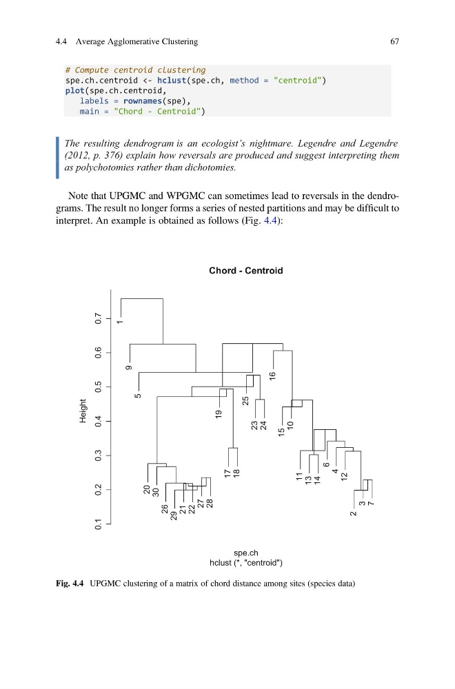
The resulting dendrogram is an ecologist’s nightmare. Legendre and Legendre
(2012, p. 376) explain how reversals are produced and suggest interpreting them
as polychotomies rather than dichotomies.
Note that UPGMC and WPGMC can sometimes lead to reversals in the dendrograms. The result no longer forms a series of nested partitions and may be difficult to
interpret. An example is obtained as follows (Fig. 4.4):
1
9
5
20
30
26
29
21
22
27
28
19
17
18
25
23
24
16
15
10
11
13
14
6
4
12
2
3
7
Chord - Centroid
spe.ch
hclust (*, "centroid")
Height
0.7
0.6
0.5
0.4
0.3
0.2
0.1
Fig. 4.4 UPGMC clustering of a matrix of chord distance among sites (species data)
4.4 Average Agglomerative Clustering
67
spe.ch.centroid <- hclust(spe.ch, method = "centroid")
plot(spe.ch.centroid,
labels = rownames(spe),
main = "Chord - Centroid")
The resulting dendrogram is an ecologist’s nightmare. Legendre and Legendre
(2012, p. 376) explain how reversals are produced and suggest interpreting them
as polychotomies rather than dichotomies.
Note that UPGMC and WPGMC can sometimes lead to reversals in the dendrograms. The result no longer forms a series of nested partitions and may be difficult to
interpret. An example is obtained as follows (Fig. 4.4):
1
9
5
20
30
26
29
21
22
27
28
19
17
18
25
23
24
16
15
10
11
13
14
6
4
12
2
3
7
Chord - Centroid
spe.ch
hclust (*, "centroid")
Height
0.7
0.6
0.5
0.4
0.3
0.2
0.1
Fig. 4.4 UPGMC clustering of a matrix of chord distance among sites (species data)
4.4 Average Agglomerative Clustering
67