

Richness difference may be caused by local species disappearances, differences in
the local abiotic conditions leading to different numbers of ecological niches, or
other ecological processes leading to communities with higher or lower numbers of
species. Nestedness is a special case of richness difference where the species at
poorer sites are a strict subset of the species present at richer sites.
This new vision of beta diversity led to the design of several methods to partition
a dissimilarity matrix into these two components. In Appendix S1 of his paper,
Legendre (2014) reviewed the development of these methods, and the main article
proposes a unifying algebraic framework to compare the published formulae.
Legendre distinguished two main families of indices, that he dubbed the Podani
and the Baselga families respectively, after the names of the authors that led two
groups of researchers who developed these indices. References can be found in the
paper. The presentation and tables below are inspired from the Legendre (2014)
paper.
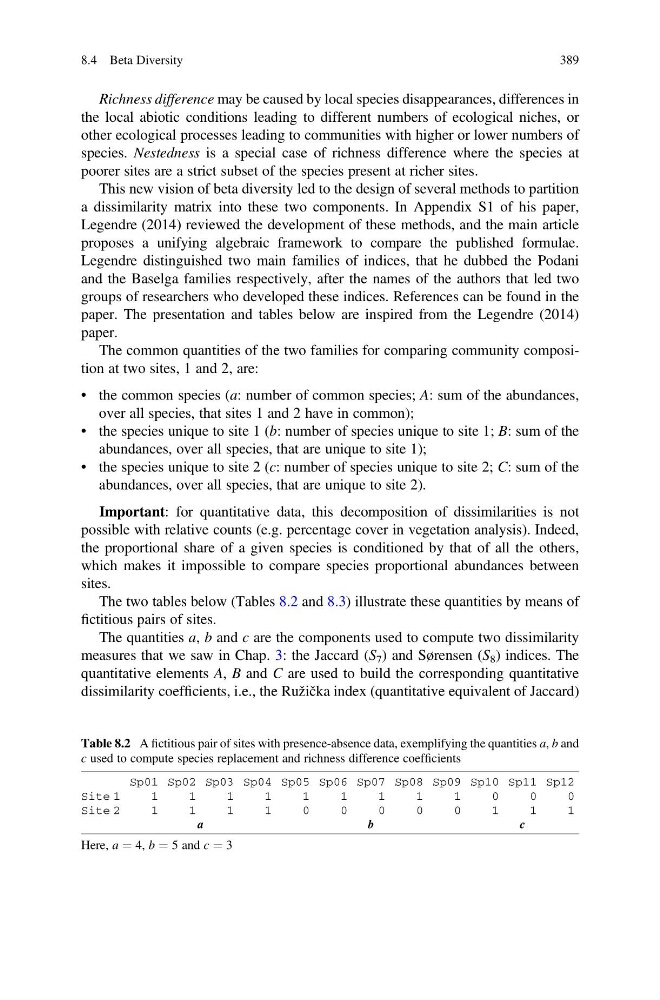
The common quantities of the two families for comparing community composition at two sites, 1 and 2, are:
• the common species (a: number of common species; A: sum of the abundances,
over all species, that sites 1 and 2 have in common);
• the species unique to site 1 (b: number of species unique to site 1; B: sum of the
abundances, over all species, that are unique to site 1);
• the species unique to site 2 (c: number of species unique to site 2; C: sum of the
abundances, over all species, that are unique to site 2).
Important: for quantitative data, this decomposition of dissimilarities is not
possible with relative counts (e.g. percentage cover in vegetation analysis). Indeed,
the proportional share of a given species is conditioned by that of all the others,
which makes it impossible to compare species proportional abundances between
sites.
The two tables below (Tables 8.2 and 8.3) illustrate these quantities by means of
fictitious pairs of sites.
The quantities a, b and c are the components used to compute two dissimilarity
measures that we saw in Chap. 3: the Jaccard (S 7 ) and Sørensen (S 8 ) indices. The
quantitative elements A, B and C are used to build the corresponding quantitative
dissimilarity coefficients, i.e., the Ružička index (quantitative equivalent of Jaccard)
Table 8.2 A fictitious pair of sites with presence-absence data, exemplifying the quantities a, b and
c used to compute species replacement and richness difference coefficients
Sp01 Sp02 Sp03 Sp04 Sp05 Sp06 Sp07 Sp08 Sp09 Sp10 Sp11 Sp12
Site 1
Site 2
1
1
1
1
1
1
1
1
1
0
1
0
1
0
1
0
1
0
0
1
0
1
0
1
a
b
c
Here, a ¼ 4, b ¼ 5 and c ¼ 3
8.4 Beta Diversity
389
the local abiotic conditions leading to different numbers of ecological niches, or
other ecological processes leading to communities with higher or lower numbers of
species. Nestedness is a special case of richness difference where the species at
poorer sites are a strict subset of the species present at richer sites.
This new vision of beta diversity led to the design of several methods to partition
a dissimilarity matrix into these two components. In Appendix S1 of his paper,
Legendre (2014) reviewed the development of these methods, and the main article
proposes a unifying algebraic framework to compare the published formulae.
Legendre distinguished two main families of indices, that he dubbed the Podani
and the Baselga families respectively, after the names of the authors that led two
groups of researchers who developed these indices. References can be found in the
paper. The presentation and tables below are inspired from the Legendre (2014)
paper.
The common quantities of the two families for comparing community composition at two sites, 1 and 2, are:
• the common species (a: number of common species; A: sum of the abundances,
over all species, that sites 1 and 2 have in common);
• the species unique to site 1 (b: number of species unique to site 1; B: sum of the
abundances, over all species, that are unique to site 1);
• the species unique to site 2 (c: number of species unique to site 2; C: sum of the
abundances, over all species, that are unique to site 2).
Important: for quantitative data, this decomposition of dissimilarities is not
possible with relative counts (e.g. percentage cover in vegetation analysis). Indeed,
the proportional share of a given species is conditioned by that of all the others,
which makes it impossible to compare species proportional abundances between
sites.
The two tables below (Tables 8.2 and 8.3) illustrate these quantities by means of
fictitious pairs of sites.
The quantities a, b and c are the components used to compute two dissimilarity
measures that we saw in Chap. 3: the Jaccard (S 7 ) and Sørensen (S 8 ) indices. The
quantitative elements A, B and C are used to build the corresponding quantitative
dissimilarity coefficients, i.e., the Ružička index (quantitative equivalent of Jaccard)
Table 8.2 A fictitious pair of sites with presence-absence data, exemplifying the quantities a, b and
c used to compute species replacement and richness difference coefficients
Sp01 Sp02 Sp03 Sp04 Sp05 Sp06 Sp07 Sp08 Sp09 Sp10 Sp11 Sp12
Site 1
Site 2
1
1
1
1
1
1
1
1
1
0
1
0
1
0
1
0
1
0
0
1
0
1
0
1
a
b
c
Here, a ¼ 4, b ¼ 5 and c ¼ 3
8.4 Beta Diversity
389