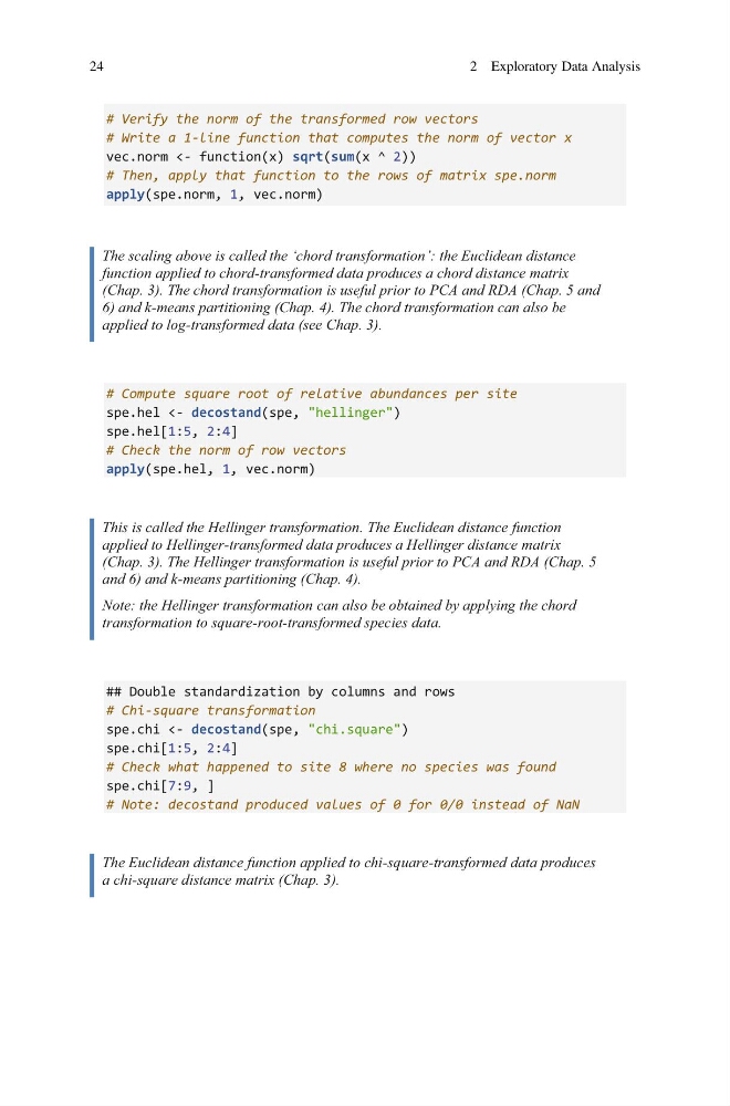
# Verify the norm of the transformed row vectors
# Write a 1-line function that computes the norm of vector x
vec.norm <- function(x) sqrt(sum(x ^ 2))
# Then, apply that function to the rows of matrix spe.norm
apply(spe.norm, 1, vec.norm)
The scaling above is called the ‘chord transformation’: the Euclidean distance
function applied to chord-transformed data produces a chord distance matrix
(Chap. 3). The chord transformation is useful prior to PCA and RDA (Chap. 5 and
6) and k-means partitioning (Chap. 4). The chord transformation can also be
applied to log-transformed data (see Chap. 3).
# Compute square root of relative abundances per site
spe.hel <- decostand(spe, "hellinger")
spe.hel[1:5, 2:4]
# Check the norm of row vectors
apply(spe.hel, 1, vec.norm)
This is called the Hellinger transformation. The Euclidean distance function
applied to Hellinger-transformed data produces a Hellinger distance matrix
(Chap. 3). The Hellinger transformation is useful prior to PCA and RDA (Chap. 5
and 6) and k-means partitioning (Chap. 4).
Note: the Hellinger transformation can also be obtained by applying the chord
transformation to square-root-transformed species data.
## Double standardization by columns and rows
# Chi-square transformation
spe.chi <- decostand(spe, "chi.square")
spe.chi[1:5, 2:4]
# Check what happened to site 8 where no species was found
spe.chi[7:9, ]
# Note: decostand produced values of 0 for 0/0 instead of NaN
The Euclidean distance function applied to chi-square-transformed data produces
a chi-square distance matrix (Chap. 3).
24
2 Exploratory Data Analysis