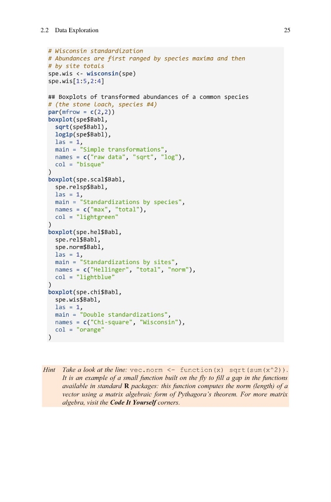
# Wisconsin standardization
# Abundances are first ranged by species maxima and then
# by site totals
spe.wis <- wisconsin(spe)
spe.wis[1:5,2:4]
## Boxplots of transformed abundances of a common species
# (the stone loach, species #4)
par(mfrow = c(2,2))
boxplot(spe$Babl,
sqrt(spe$Babl),
log1p(spe$Babl),
las = 1,
main = "Simple transformations",
names = c("raw data", "sqrt", "log"),
col = "bisque"
)
boxplot(spe.scal$Babl,
spe.relsp$Babl,
las = 1,
main = "Standardizations by species",
names = c("max", "total"),
col = "lightgreen"
)
boxplot(spe.hel$Babl,
spe.rel$Babl,
spe.norm$Babl,
las = 1,
main = "Standardizations by sites",
names = c("Hellinger", "total", "norm"),
col = "lightblue"
)
boxplot(spe.chi$Babl,
spe.wis$Babl,
las = 1,
main = "Double standardizations",
names = c("Chi-square", "Wisconsin"),
col = "orange"
)
Hint Take a look at the line: vec.norm <- function(x) sqrt(sum(x^2)).
It is an example of a small function built on the fly to fill a gap in the functions
available in standard R packages: this function computes the norm (length) of a
vector using a matrix algebraic form of Pythagora’s theorem. For more matrix
algebra, visit the Code It Yourself corners.
2.2 Data Exploration
25