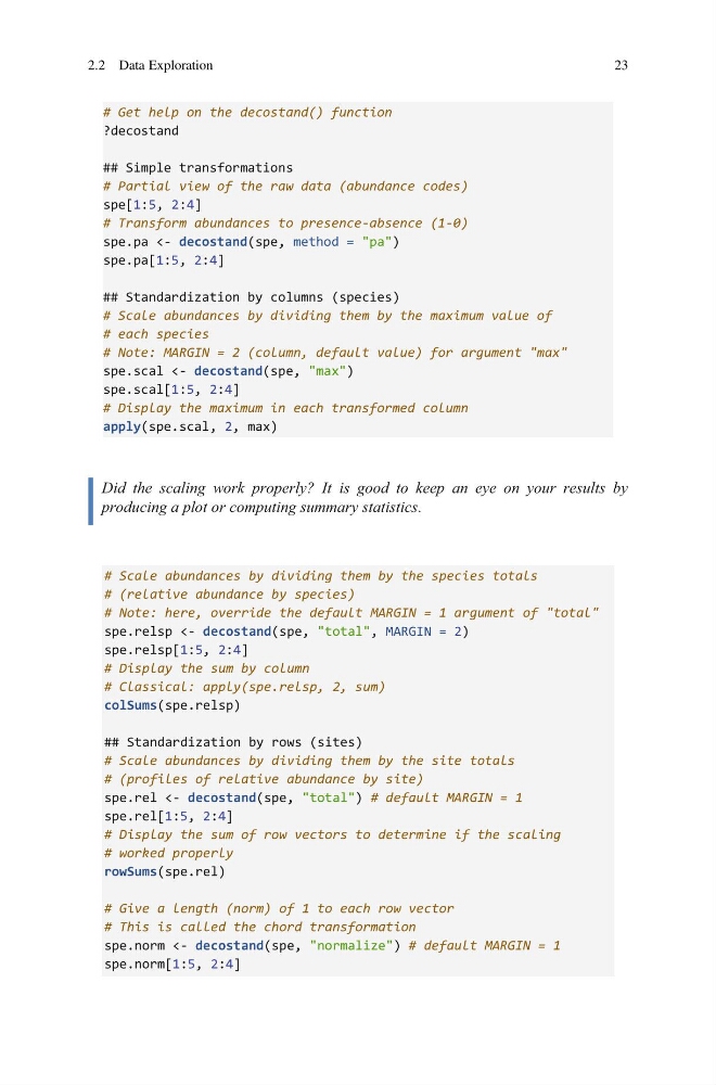
# Get help on the decostand() function
?decostand
## Simple transformations
# Partial view of the raw data (abundance codes)
spe[1:5, 2:4]
# Transform abundances to presence-absence (1-0)
spe.pa <- decostand(spe, method = "pa")
spe.pa[1:5, 2:4]
## Standardization by columns (species)
# Scale abundances by dividing them by the maximum value of
# each species
# Note: MARGIN = 2 (column, default value) for argument "max"
spe.scal <- decostand(spe, "max")
spe.scal[1:5, 2:4]
# Display the maximum in each transformed column
apply(spe.scal, 2, max)
Did the scaling work properly? It is good to keep an eye on your results by
producing a plot or computing summary statistics.
# Scale abundances by dividing them by the species totals
# (relative abundance by species)
# Note: here, override the default MARGIN = 1 argument of "total"
spe.relsp <- decostand(spe, "total", MARGIN = 2)
spe.relsp[1:5, 2:4]
# Display the sum by column
# Classical: apply(spe.relsp, 2, sum)
colSums(spe.relsp)
## Standardization by rows (sites)
# Scale abundances by dividing them by the site totals
# (profiles of relative abundance by site)
spe.rel <- decostand(spe, "total") # default MARGIN = 1
spe.rel[1:5, 2:4]
# Display the sum of row vectors to determine if the scaling
# worked properly
rowSums(spe.rel)
# Give a length (norm) of 1 to each row vector
# This is called the chord transformation
spe.norm <- decostand(spe, "normalize") # default MARGIN = 1
spe.norm[1:5, 2:4]
2.2 Data Exploration
23