

These MEM results show that the whole process of selecting and fine-tuning a
spatial model, cumbersome as it may seem, can end up with an efficient and
parsimonious set of spatial variables.
7.4.3.3 Other Types of Connectivity Matrices
In some special cases where one has a specific model of spatial connections in mind,
it is useless to go through the automatic procedure shown above, which finds the best
model among multiple possibilities. The present section shows how to construct
connectivity matrices of several types by hand.
Depending on the context (hypotheses, data), researchers may need connecting
schemes that are more or less dense or even locally customized. In such cases, the
use of an automatic procedure including the computation of a minimum spanning
tree as in the dbMEM procedure presented in Sect. 7.4.2.1, or of a Delaunay
connectivity matrix, may not be appropriate. Ecological reasons include topographical structure of the sampling area (including possible barriers), dispersion ability of
the organisms, permeability of some types of substrates, and so on.
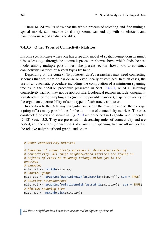
In addition to the Delaunay triangulation used in the example above, the package
spdep offers many possibilities for the definition of connectivity matrices. The ones
constructed below and shown in Fig. 7.10 are described in Legendre and Legendre
(2012) Sect. 13.3. They are presented in decreasing order of connectivity and are
nested, i.e., the edges (connections) of a minimum spanning tree are all included in
the relative neighbourhood graph, and so on.
# Other connectivity matrices
# Examples of connectivity matrices in decreasing order of
# connectivity. All these neighbourhood matrices are stored in
# objects of class nb Delaunay triangulation (as in the
previous
# example)
mite.del <- tri2nb(mite.xy)
# Gabriel graph
mite.gab <- graph2nb(gabrielneigh(as.matrix(mite.xy)), sym = TRUE)
# Relative neighbourhood
mite.rel <- graph2nb(relativeneigh(as.matrix(mite.xy)), sym = TRUE)
# Minimum spanning tree
mite.mst <- mst.nb(dist(mite.xy))
All these neighbourhood matrices are stored in objects of class nb.
342
7 Spatial Analysis of Ecological Data
spatial model, cumbersome as it may seem, can end up with an efficient and
parsimonious set of spatial variables.
7.4.3.3 Other Types of Connectivity Matrices
In some special cases where one has a specific model of spatial connections in mind,
it is useless to go through the automatic procedure shown above, which finds the best
model among multiple possibilities. The present section shows how to construct
connectivity matrices of several types by hand.
Depending on the context (hypotheses, data), researchers may need connecting
schemes that are more or less dense or even locally customized. In such cases, the
use of an automatic procedure including the computation of a minimum spanning
tree as in the dbMEM procedure presented in Sect. 7.4.2.1, or of a Delaunay
connectivity matrix, may not be appropriate. Ecological reasons include topographical structure of the sampling area (including possible barriers), dispersion ability of
the organisms, permeability of some types of substrates, and so on.
In addition to the Delaunay triangulation used in the example above, the package
spdep offers many possibilities for the definition of connectivity matrices. The ones
constructed below and shown in Fig. 7.10 are described in Legendre and Legendre
(2012) Sect. 13.3. They are presented in decreasing order of connectivity and are
nested, i.e., the edges (connections) of a minimum spanning tree are all included in
the relative neighbourhood graph, and so on.
# Other connectivity matrices
# Examples of connectivity matrices in decreasing order of
# connectivity. All these neighbourhood matrices are stored in
# objects of class nb Delaunay triangulation (as in the
previous
# example)
mite.del <- tri2nb(mite.xy)
# Gabriel graph
mite.gab <- graph2nb(gabrielneigh(as.matrix(mite.xy)), sym = TRUE)
# Relative neighbourhood
mite.rel <- graph2nb(relativeneigh(as.matrix(mite.xy)), sym = TRUE)
# Minimum spanning tree
mite.mst <- mst.nb(dist(mite.xy))
All these neighbourhood matrices are stored in objects of class nb.
342
7 Spatial Analysis of Ecological Data