

# Plots of the connectivity matrices
par(mfrow = c(2,2))
plot(mite.del, mite.xy, col = "red", pch = 20, cex = 1)
title(main = "Delaunay triangulation ")
plot(mite.gab, mite.xy, col = "purple", pch = 20, cex = 1)
title(main = "Gabriel graph")
plot(mite.rel, mite.xy, col = "dark green", pch = 20, cex = 1)
title(main = "Relative neighbourhood")
plot(mite.mst, mite.xy, col = "brown", pch = 20, cex = 1)
title(main = "Minimum spanning tree")
Some of these matrices may contain unwanted links (for instance along the
borders of the areas). These can be edited out either interactively or by command
lines:
# Link editing
# 1. Interactive:
dev.new(title = "Delaunay triangulation")
plot(mite.del, mite.xy, col = "red", pch = 20, cex = 2)
title(main = "Delaunay triangulation")
mite.del2 <- edit.nb(mite.del, mite.xy)
Delaunay triangulation
Gabriel graph
Relative neighbourhood
Minimum spanning tree
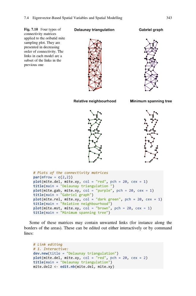
Fig. 7.10 Four types of
connectivity matrices
applied to the oribatid mite
sampling plot. They are
presented in decreasing
order of connectivity. The
links in each model are a
subset of the links in the
previous one
7.4 Eigenvector-Based Spatial Variables and Spatial Modelling
343
par(mfrow = c(2,2))
plot(mite.del, mite.xy, col = "red", pch = 20, cex = 1)
title(main = "Delaunay triangulation ")
plot(mite.gab, mite.xy, col = "purple", pch = 20, cex = 1)
title(main = "Gabriel graph")
plot(mite.rel, mite.xy, col = "dark green", pch = 20, cex = 1)
title(main = "Relative neighbourhood")
plot(mite.mst, mite.xy, col = "brown", pch = 20, cex = 1)
title(main = "Minimum spanning tree")
Some of these matrices may contain unwanted links (for instance along the
borders of the areas). These can be edited out either interactively or by command
lines:
# Link editing
# 1. Interactive:
dev.new(title = "Delaunay triangulation")
plot(mite.del, mite.xy, col = "red", pch = 20, cex = 2)
title(main = "Delaunay triangulation")
mite.del2 <- edit.nb(mite.del, mite.xy)
Delaunay triangulation
Gabriel graph
Relative neighbourhood
Minimum spanning tree
Fig. 7.10 Four types of
connectivity matrices
applied to the oribatid mite
sampling plot. They are
presented in decreasing
order of connectivity. The
links in each model are a
subset of the links in the
previous one
7.4 Eigenvector-Based Spatial Variables and Spatial Modelling
343