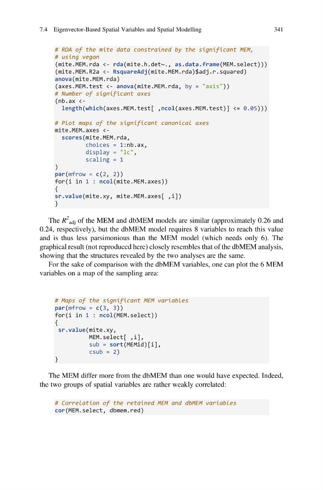
# RDA of the mite data constrained by the significant MEM,
# using vegan
(mite.MEM.rda <- rda(mite.h.det~., as.data.frame(MEM.select)))
(mite.MEM.R2a <- RsquareAdj(mite.MEM.rda)$adj.r.squared)
anova(mite.MEM.rda)
(axes.MEM.test <- anova(mite.MEM.rda, by = "axis"))
# Number of significant axes
(nb.ax # Plot maps of the significant canonical axes
mite.MEM.axes choices = 1:nb.ax,
display = "lc",
scaling = 1
)
par(mfrow = c(2, 2))
for(i in 1 : ncol(mite.MEM.axes))
{
sr.value(mite.xy, mite.MEM.axes[ ,i])
}
The R
2
adj of the MEM and dbMEM models are similar (approximately 0.26 and
0.24, respectively), but the dbMEM model requires 8 variables to reach this value
and is thus less parsimonious than the MEM model (which needs only 6). The
graphical result (not reproduced here) closely resembles that of the dbMEM analysis,
showing that the structures revealed by the two analyses are the same.
For the sake of comparison with the dbMEM variables, one can plot the 6 MEM
variables on a map of the sampling area:
# Maps of the significant MEM variables
par(mfrow = c(3, 3))
for(i in 1 : ncol(MEM.select))
{
sr.value(mite.xy,
MEM.select[ ,i],
sub = sort(MEMid)[i],
csub = 2)
}
The MEM differ more from the dbMEM than one would have expected. Indeed,
the two groups of spatial variables are rather weakly correlated:
# Correlation of the retained MEM and dbMEM variables
cor(MEM.select, dbmem.red)
7.4 Eigenvector-Based Spatial Variables and Spatial Modelling
341