With an AICc of À100.96, this is the best result of all our attempts in terms of
AICc. We can therefore extract this champion model, which contains 6 selected
MEM variables, from the output object:
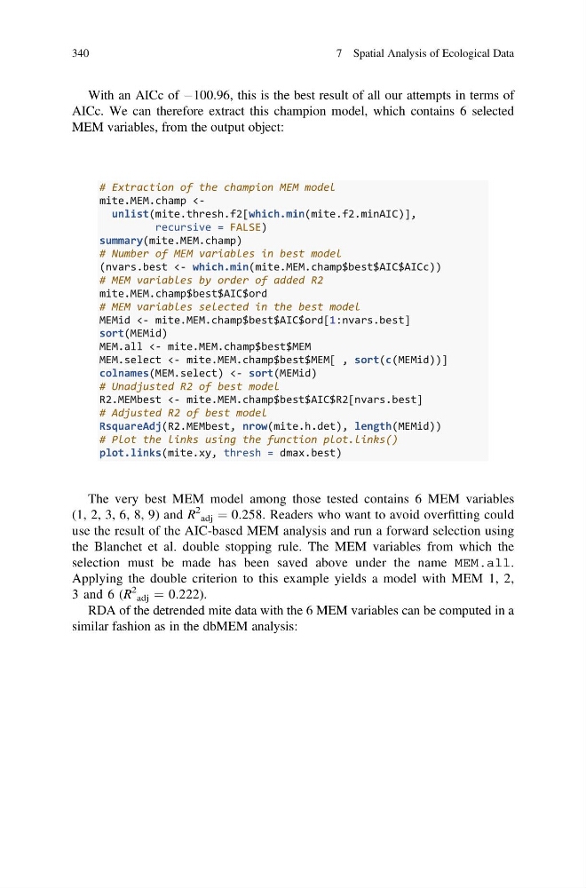
# Extraction of the champion MEM model
mite.MEM.champ recursive = FALSE)
summary(mite.MEM.champ)
# Number of MEM variables in best model
(nvars.best <- which.min(mite.MEM.champ$best$AIC$AICc))
# MEM variables by order of added R2
mite.MEM.champ$best$AIC$ord
# MEM variables selected in the best model
MEMid <- mite.MEM.champ$best$AIC$ord[1:nvars.best]
sort(MEMid)
MEM.all <- mite.MEM.champ$best$MEM
MEM.select <- mite.MEM.champ$best$MEM[ , sort(c(MEMid))]
colnames(MEM.select) <- sort(MEMid)
# Unadjusted R2 of best model
R2.MEMbest <- mite.MEM.champ$best$AIC$R2[nvars.best]
# Adjusted R2 of best model
RsquareAdj(R2.MEMbest, nrow(mite.h.det), length(MEMid))
# Plot the links using the function plot.links()
plot.links(mite.xy, thresh = dmax.best)
The very best MEM model among those tested contains 6 MEM variables
(1, 2, 3, 6, 8, 9) and R
2
adj ¼ 0.258. Readers who want to avoid overfitting could
use the result of the AIC-based MEM analysis and run a forward selection using
the Blanchet et al. double stopping rule. The MEM variables from which the
selection must be made has been saved above under the name MEM.all.
Applying the double criterion to this example yields a model with MEM 1, 2,
3 and 6 (R
2
adj ¼ 0.222).
RDA of the detrended mite data with the 6 MEM variables can be computed in a
similar fashion as in the dbMEM analysis:
340
7 Spatial Analysis of Ecological Data