

The dbMEM analysis of the detrended mite data explained 24.18% of the
variance (see mite.fwd.R2a, the adjusted R
2 obtained with the 8 dbMEM variables retained by forward selection). Three canonical axes, explaining
24.18 Â 0.8895
3
¼ 21.5% of the total variance, are significant; their fitted site
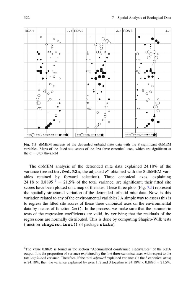
scores have been plotted on a map of the sites. These three plots (Fig. 7.5) represent
the spatially structured variation of the detrended oribatid mite data. Now, is this
variation related to any of the environmental variables? A simple way to assess this is
to regress the fitted site scores of these three canonical axes on the environmental
data by means of function lm(). In the process, we make sure that the parametric
tests of the regression coefficients are valid, by verifying that the residuals of the
regressions are normally distributed. This is done by computing Shapiro-Wilk tests
(function shapiro.test() of package stats).
d = 1
RDA 1
-0.25
-0.15
-0.05 0.05 0.15
0.25
d = 1
RDA 2
d = 1
RDA 3
-0.075
-0.025 0.025 0.075
-0.15
-0.05
0.05
0.15
Fig. 7.5 dbMEM analysis of the detrended oribatid mite data with the 8 significant dbMEM
variables. Maps of the fitted site scores of the first three canonical axes, which are significant at
the α ¼ 0.05 threshold
3 The value 0.8895 is found in the section “Accumulated constrained eigenvalues” of the RDA
output. It is the proportion of variance explained by the first three canonical axes with respect to the
total explained variance. Therefore, if the total adjusted explained variance (in the 8 canonical axes)
is 24.18%, then the variance explained by axes 1, 2 and 3 together is 24.18% Â 0.8895 ¼ 21.5%.
322
7 Spatial Analysis of Ecological Data
variance (see mite.fwd.R2a, the adjusted R
2 obtained with the 8 dbMEM variables retained by forward selection). Three canonical axes, explaining
24.18 Â 0.8895
3
¼ 21.5% of the total variance, are significant; their fitted site
scores have been plotted on a map of the sites. These three plots (Fig. 7.5) represent
the spatially structured variation of the detrended oribatid mite data. Now, is this
variation related to any of the environmental variables? A simple way to assess this is
to regress the fitted site scores of these three canonical axes on the environmental
data by means of function lm(). In the process, we make sure that the parametric
tests of the regression coefficients are valid, by verifying that the residuals of the
regressions are normally distributed. This is done by computing Shapiro-Wilk tests
(function shapiro.test() of package stats).
d = 1
RDA 1
-0.25
-0.15
-0.05 0.05 0.15
0.25
d = 1
RDA 2
d = 1
RDA 3
-0.075
-0.025 0.025 0.075
-0.15
-0.05
0.05
0.15
Fig. 7.5 dbMEM analysis of the detrended oribatid mite data with the 8 significant dbMEM
variables. Maps of the fitted site scores of the first three canonical axes, which are significant at
the α ¼ 0.05 threshold
3 The value 0.8895 is found in the section “Accumulated constrained eigenvalues” of the RDA
output. It is the proportion of variance explained by the first three canonical axes with respect to the
total explained variance. Therefore, if the total adjusted explained variance (in the 8 canonical axes)
is 24.18%, then the variance explained by axes 1, 2 and 3 together is 24.18% Â 0.8895 ¼ 21.5%.
322
7 Spatial Analysis of Ecological Data