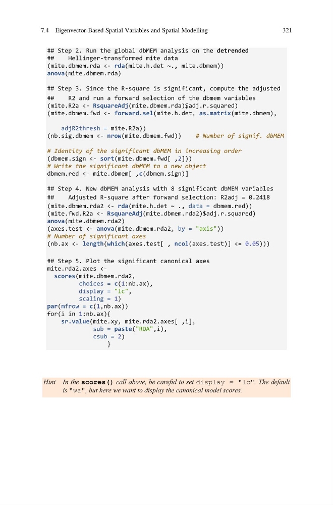
## Step 2. Run the global dbMEM analysis on the detrended
##
Hellinger-transformed mite data
(mite.dbmem.rda <- rda(mite.h.det ~., mite.dbmem))
anova(mite.dbmem.rda)
## Step 3. Since the R-square is significant, compute the adjusted
##
R2 and run a forward selection of the dbmem variables
(mite.R2a <- RsquareAdj(mite.dbmem.rda)$adj.r.squared)
(mite.dbmem.fwd <- forward.sel(mite.h.det, as.matrix(mite.dbmem),
adjR2thresh = mite.R2a))
(nb.sig.dbmem <- nrow(mite.dbmem.fwd))
# Number of signif. dbMEM
# Identity of the significant dbMEM in increasing order
(dbmem.sign <- sort(mite.dbmem.fwd[ ,2]))
# Write the significant dbMEM to a new object
dbmem.red <- mite.dbmem[ ,c(dbmem.sign)]
## Step 4. New dbMEM analysis with 8 significant dbMEM variables
##
Adjusted R-square after forward selection: R2adj = 0.2418
(mite.dbmem.rda2 <- rda(mite.h.det ~ ., data = dbmem.red))
(mite.fwd.R2a <- RsquareAdj(mite.dbmem.rda2)$adj.r.squared)
anova(mite.dbmem.rda2)
(axes.test <- anova(mite.dbmem.rda2, by = "axis"))
# Number of significant axes
(nb.ax <- length(which(axes.test[ , ncol(axes.test)] <= 0.05)))
## Step 5. Plot the significant canonical axes
mite.rda2.axes choices = c(1:nb.ax),
display = "lc",
scaling = 1)
par(mfrow = c(1,nb.ax))
for(i in 1:nb.ax){
sr.value(mite.xy, mite.rda2.axes[ ,i],
sub = paste("RDA",i),
csub = 2)
}
Hint In the scores() call above, be careful to set display = "lc". The default
is "wa", but here we want to display the canonical model scores.
7.4 Eigenvector-Based Spatial Variables and Spatial Modelling
321