

Since both matrices involved contain species data, it is preferable to use a method
that respects this particularity also for the explanatory matrix, as co-correspondence
analysis does. The two reasons invoked by its authors are (1) CCA (and RDA) can
only be used when the number of explanatory variables is smaller than the number of
sites (which is often not the case with community data), and (2) the linear combinations of explanatory variables are not well suited to cases where these variables are
themselves species data with many zeros and unimodal distributions with respect to
the environment. ter Braak and Schaffers (2004) present the mathematics of the
method in detail. Very briefly: the first ordination axis of symmetric and asymmetric
CoCA is obtained by weighted averages, where (quoting the authors) “the species
scores of one set are obtained as weighted averages of the other set’s site scores
[and] the site scores are weighted averages of the species scores of their own set”.
Then, in symmetric CoCA, the next axes are extracted in the same way, with the
successive species scores uncorrelated with the previous ones. In asymmetric CoCA,
the successive axes are constructed such that “the site scores derived from the
predictor variables [are] uncorrelated with the previously derived site scores”.
The number of axes to interpret can be assessed either by cross-validation (details
in the paper) or by a permutation test.
Symmetric and asymmetric co-correspondence analysis can be computed with an
R package called cocorresp. Here we present one of the examples proposed in
the documentation file of the function. The example, also treated in ter Braak and
Schaffers’ (2004) paper, deals with bryophytes and vascular plants in Carpathian
spring meadows. The data set comprises 70 sites and the species of both communities that are present in at least 5 sites, i.e., 30 bryophyte and 123 vascular plant
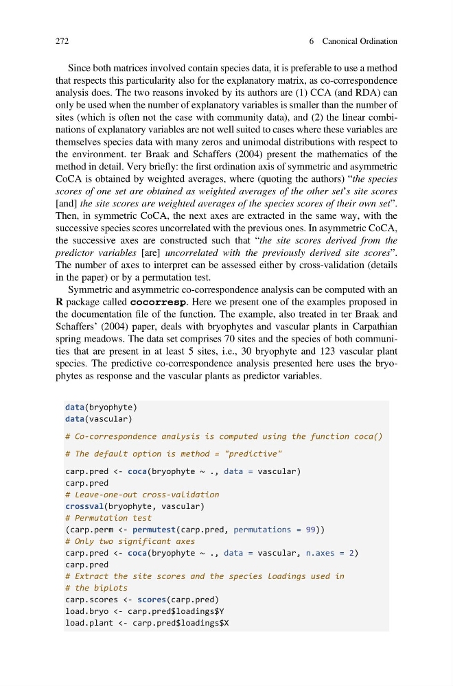
species. The predictive co-correspondence analysis presented here uses the bryophytes as response and the vascular plants as predictor variables.
data(bryophyte)
data(vascular)
# Co-correspondence analysis is computed using the function coca()
# The default option is method = "predictive"
carp.pred <- coca(bryophyte ~ ., data = vascular)
carp.pred
# Leave-one-out cross-validation
crossval(bryophyte, vascular)
# Permutation test
(carp.perm <- permutest(carp.pred, permutations = 99))
# Only two significant axes
carp.pred <- coca(bryophyte ~ ., data = vascular, n.axes = 2)
carp.pred
# Extract the site scores and the species loadings used in
# the biplots
carp.scores <- scores(carp.pred)
load.bryo <- carp.pred$loadings$Y
load.plant <- carp.pred$loadings$X
272
6 Canonical Ordination
that respects this particularity also for the explanatory matrix, as co-correspondence
analysis does. The two reasons invoked by its authors are (1) CCA (and RDA) can
only be used when the number of explanatory variables is smaller than the number of
sites (which is often not the case with community data), and (2) the linear combinations of explanatory variables are not well suited to cases where these variables are
themselves species data with many zeros and unimodal distributions with respect to
the environment. ter Braak and Schaffers (2004) present the mathematics of the
method in detail. Very briefly: the first ordination axis of symmetric and asymmetric
CoCA is obtained by weighted averages, where (quoting the authors) “the species
scores of one set are obtained as weighted averages of the other set’s site scores
[and] the site scores are weighted averages of the species scores of their own set”.
Then, in symmetric CoCA, the next axes are extracted in the same way, with the
successive species scores uncorrelated with the previous ones. In asymmetric CoCA,
the successive axes are constructed such that “the site scores derived from the
predictor variables [are] uncorrelated with the previously derived site scores”.
The number of axes to interpret can be assessed either by cross-validation (details
in the paper) or by a permutation test.
Symmetric and asymmetric co-correspondence analysis can be computed with an
R package called cocorresp. Here we present one of the examples proposed in
the documentation file of the function. The example, also treated in ter Braak and
Schaffers’ (2004) paper, deals with bryophytes and vascular plants in Carpathian
spring meadows. The data set comprises 70 sites and the species of both communities that are present in at least 5 sites, i.e., 30 bryophyte and 123 vascular plant
species. The predictive co-correspondence analysis presented here uses the bryophytes as response and the vascular plants as predictor variables.
data(bryophyte)
data(vascular)
# Co-correspondence analysis is computed using the function coca()
# The default option is method = "predictive"
carp.pred <- coca(bryophyte ~ ., data = vascular)
carp.pred
# Leave-one-out cross-validation
crossval(bryophyte, vascular)
# Permutation test
(carp.perm <- permutest(carp.pred, permutations = 99))
# Only two significant axes
carp.pred <- coca(bryophyte ~ ., data = vascular, n.axes = 2)
carp.pred
# Extract the site scores and the species loadings used in
# the biplots
carp.scores <- scores(carp.pred)
load.bryo <- carp.pred$loadings$Y
load.plant <- carp.pred$loadings$X
272
6 Canonical Ordination