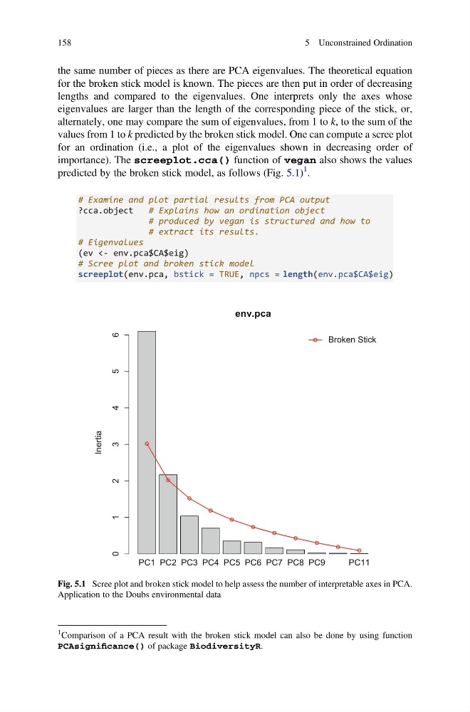
the same number of pieces as there are PCA eigenvalues. The theoretical equation
for the broken stick model is known. The pieces are then put in order of decreasing
lengths and compared to the eigenvalues. One interprets only the axes whose
eigenvalues are larger than the length of the corresponding piece of the stick, or,
alternately, one may compare the sum of eigenvalues, from 1 to k, to the sum of the
values from 1 to k predicted by the broken stick model. One can compute a scree plot
for an ordination (i.e., a plot of the eigenvalues shown in decreasing order of
importance). The screeplot.cca() function of vegan also shows the values
predicted by the broken stick model, as follows (Fig. 5.1)
1 .
# Examine and plot partial results from PCA output
?cca.object
# Explains how an ordination object
# produced by vegan is structured and how to
# extract its results.
# Eigenvalues
(ev <- env.pca$CA$eig)
# Scree plot and broken stick model
screeplot(env.pca, bstick = TRUE, npcs = length(env.pca$CA$eig)
PC1 PC2 PC3 PC4 PC5 PC6 PC7 PC8 PC9
PC11
env.pca
Inertia
0
1
2
3
4
5
6
Broken Stick
Fig. 5.1 Scree plot and broken stick model to help assess the number of interpretable axes in PCA.
Application to the Doubs environmental data
1 Comparison of a PCA result with the broken stick model can also be done by using function
PCAsignificance() of package BiodiversityR.
158
5 Unconstrained Ordination