

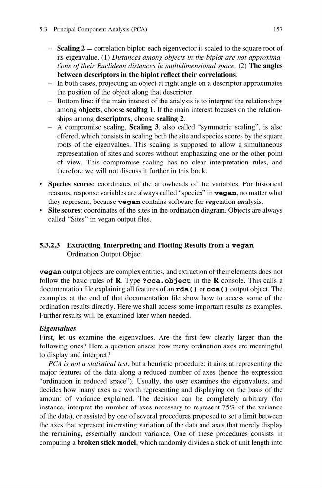
– Scaling 2 ¼ correlation biplot: each eigenvector is scaled to the square root of
its eigenvalue. (1) Distances among objects in the biplot are not approximations of their Euclidean distances in multidimensional space. (2) The angles
between descriptors in the biplot reflect their correlations.
– In both cases, projecting an object at right angle on a descriptor approximates
the position of the object along that descriptor.
– Bottom line: if the main interest of the analysis is to interpret the relationships
among objects, choose scaling 1. If the main interest focuses on the relationships among descriptors, choose scaling 2.
– A compromise scaling, Scaling 3, also called “symmetric scaling”, is also
offered, which consists in scaling both the site and species scores by the square
roots of the eigenvalues. This scaling is supposed to allow a simultaneous
representation of sites and scores without emphasizing one or the other point
of view. This compromise scaling has no clear interpretation rules, and
therefore we will not discuss it further in this book.
• Species scores: coordinates of the arrowheads of the variables. For historical
reasons, response variables are always called “species” in vegan, no matter what
they represent, because vegan contains software for vegetation analysis.
• Site scores: coordinates of the sites in the ordination diagram. Objects are always
called “Sites” in vegan output files.
5.3.2.3 Extracting, Interpreting and Plotting Results from a vegan
Ordination Output Object
vegan output objects are complex entities, and extraction of their elements does not
follow the basic rules of R. Type ?cca.object in the R console. This calls a
documentation file explaining all features of an rda() or cca() output object. The
examples at the end of that documentation file show how to access some of the
ordination results directly. Here we shall access some important results as examples.
Further results will be examined later when needed.
Eigenvalues
First, let us examine the eigenvalues. Are the first few clearly larger than the
following ones? Here a question arises: how many ordination axes are meaningful
to display and interpret?
PCA is not a statistical test, but a heuristic procedure; it aims at representing the
major features of the data along a reduced number of axes (hence the expression
“ordination in reduced space”). Usually, the user examines the eigenvalues, and
decides how many axes are worth representing and displaying on the basis of the
amount of variance explained. The decision can be completely arbitrary (for
instance, interpret the number of axes necessary to represent 75% of the variance
of the data), or assisted by one of several procedures proposed to set a limit between
the axes that represent interesting variation of the data and axes that merely display
the remaining, essentially random variance. One of these procedures consists in
computing a broken stick model, which randomly divides a stick of unit length into
5.3 Principal Component Analysis (PCA)
157
its eigenvalue. (1) Distances among objects in the biplot are not approximations of their Euclidean distances in multidimensional space. (2) The angles
between descriptors in the biplot reflect their correlations.
– In both cases, projecting an object at right angle on a descriptor approximates
the position of the object along that descriptor.
– Bottom line: if the main interest of the analysis is to interpret the relationships
among objects, choose scaling 1. If the main interest focuses on the relationships among descriptors, choose scaling 2.
– A compromise scaling, Scaling 3, also called “symmetric scaling”, is also
offered, which consists in scaling both the site and species scores by the square
roots of the eigenvalues. This scaling is supposed to allow a simultaneous
representation of sites and scores without emphasizing one or the other point
of view. This compromise scaling has no clear interpretation rules, and
therefore we will not discuss it further in this book.
• Species scores: coordinates of the arrowheads of the variables. For historical
reasons, response variables are always called “species” in vegan, no matter what
they represent, because vegan contains software for vegetation analysis.
• Site scores: coordinates of the sites in the ordination diagram. Objects are always
called “Sites” in vegan output files.
5.3.2.3 Extracting, Interpreting and Plotting Results from a vegan
Ordination Output Object
vegan output objects are complex entities, and extraction of their elements does not
follow the basic rules of R. Type ?cca.object in the R console. This calls a
documentation file explaining all features of an rda() or cca() output object. The
examples at the end of that documentation file show how to access some of the
ordination results directly. Here we shall access some important results as examples.
Further results will be examined later when needed.
Eigenvalues
First, let us examine the eigenvalues. Are the first few clearly larger than the
following ones? Here a question arises: how many ordination axes are meaningful
to display and interpret?
PCA is not a statistical test, but a heuristic procedure; it aims at representing the
major features of the data along a reduced number of axes (hence the expression
“ordination in reduced space”). Usually, the user examines the eigenvalues, and
decides how many axes are worth representing and displaying on the basis of the
amount of variance explained. The decision can be completely arbitrary (for
instance, interpret the number of axes necessary to represent 75% of the variance
of the data), or assisted by one of several procedures proposed to set a limit between
the axes that represent interesting variation of the data and axes that merely display
the remaining, essentially random variance. One of these procedures consists in
computing a broken stick model, which randomly divides a stick of unit length into
5.3 Principal Component Analysis (PCA)
157