

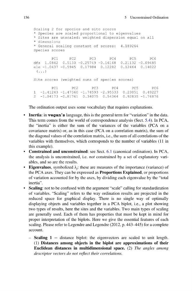
Scaling 2 for species and site scores
* Species are scaled proportional to eigenvalues
* Sites are unscaled: weighted dispersion equal on all
* dimensions
* General scaling constant of scores: 4.189264
Species scores
PC1
PC2
PC3
PC4
PC5
PC6
dfs 1.0842 0.5150 -0.25749 -0.16168 0.21132 -0.09485
ele -1.0437 -0.5945 0.17984 0.12282 0.12464 0.14022
(...)
Site scores (weighted sums of species scores)
PC1
PC2
PC3
PC4
PC5
PC6
1 -1.41243 -1.47560 -1.74593 -2.95533 0.23051 0.49227
2 -1.04173 -0.81761 0.34075 0.54364 0.92835 -1.76876
The ordination output uses some vocabulary that requires explanations.
• Inertia: in vegan’s language, this is the general term for “variation” in the data.
This term comes from the world of correspondence analysis (Sect. 5.4). In PCA,
the “inertia” is either the sum of the variances of the variables (PCA on a
covariance matrix) or, as in this case (PCA on a correlation matrix), the sum of
the diagonal values of the correlation matrix, i.e., the sum of all correlations of the
variables with themselves, which corresponds to the number of variables (11 in
this example).
• Constrained and unconstrained: see Sect. 6.1 (canonical ordination). In PCA,
the analysis is unconstrained, i.e. not constrained by a set of explanatory variables, and so are the results.
• Eigenvalues, symbolized λ j : these are measures of the importance (variance) of
the PCA axes. They can be expressed as Proportions Explained, or proportions
of variation accounted for by the axes, by dividing each eigenvalue by the “total
inertia”.
• Scaling: not to be confused with the argument “scale” calling for standardization
of variables. “Scaling” refers to the way ordination results are projected in the
reduced space for graphical display. There is no single way of optimally
displaying objects and variables together in a PCA biplot, i.e., a plot showing
two types of results, here the sites and the variables. Two main types of scaling
are generally used. Each of them has properties that must be kept in mind for
proper interpretation of the biplots. Here we give the essential features of each
scaling. Please refer to Legendre and Legendre (2012, p. 443–445) for a complete
account.
– Scaling 1 ¼ distance biplot: the eigenvectors are scaled to unit length.
(1) Distances among objects in the biplot are approximations of their
Euclidean distances in multidimensional space. (2) The angles among
descriptor vectors do not reflect their correlations.
156
5 Unconstrained Ordination
* Species are scaled proportional to eigenvalues
* Sites are unscaled: weighted dispersion equal on all
* dimensions
* General scaling constant of scores: 4.189264
Species scores
PC1
PC2
PC3
PC4
PC5
PC6
dfs 1.0842 0.5150 -0.25749 -0.16168 0.21132 -0.09485
ele -1.0437 -0.5945 0.17984 0.12282 0.12464 0.14022
(...)
Site scores (weighted sums of species scores)
PC1
PC2
PC3
PC4
PC5
PC6
1 -1.41243 -1.47560 -1.74593 -2.95533 0.23051 0.49227
2 -1.04173 -0.81761 0.34075 0.54364 0.92835 -1.76876
The ordination output uses some vocabulary that requires explanations.
• Inertia: in vegan’s language, this is the general term for “variation” in the data.
This term comes from the world of correspondence analysis (Sect. 5.4). In PCA,
the “inertia” is either the sum of the variances of the variables (PCA on a
covariance matrix) or, as in this case (PCA on a correlation matrix), the sum of
the diagonal values of the correlation matrix, i.e., the sum of all correlations of the
variables with themselves, which corresponds to the number of variables (11 in
this example).
• Constrained and unconstrained: see Sect. 6.1 (canonical ordination). In PCA,
the analysis is unconstrained, i.e. not constrained by a set of explanatory variables, and so are the results.
• Eigenvalues, symbolized λ j : these are measures of the importance (variance) of
the PCA axes. They can be expressed as Proportions Explained, or proportions
of variation accounted for by the axes, by dividing each eigenvalue by the “total
inertia”.
• Scaling: not to be confused with the argument “scale” calling for standardization
of variables. “Scaling” refers to the way ordination results are projected in the
reduced space for graphical display. There is no single way of optimally
displaying objects and variables together in a PCA biplot, i.e., a plot showing
two types of results, here the sites and the variables. Two main types of scaling
are generally used. Each of them has properties that must be kept in mind for
proper interpretation of the biplots. Here we give the essential features of each
scaling. Please refer to Legendre and Legendre (2012, p. 443–445) for a complete
account.
– Scaling 1 ¼ distance biplot: the eigenvectors are scaled to unit length.
(1) Distances among objects in the biplot are approximations of their
Euclidean distances in multidimensional space. (2) The angles among
descriptor vectors do not reflect their correlations.
156
5 Unconstrained Ordination