Biplots of sites and variables
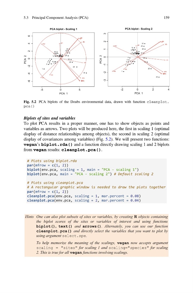
To plot PCA results in a proper manner, one has to show objects as points and
variables as arrows. Two plots will be produced here, the first in scaling 1 (optimal
display of distance relationships among objects), the second in scaling 2 (optimal
display of covariances among variables) (Fig. 5.2). We will present two functions:
vegan’s biplot.rda() and a function directly drawing scaling 1 and 2 biplots
from vegan results: cleanplot.pca().
# Plots using biplot.rda
par(mfrow = c(1, 2))
biplot(env.pca, scaling = 1, main = "PCA - scaling 1")
biplot(env.pca, main = "PCA - scaling 2") # Default scaling 2
# Plots using cleanplot.pca
# A rectangular graphic window is needed to draw the plots together
par(mfrow = c(1, 2))
cleanplot.pca(env.pca, scaling = 1, mar.percent = 0.08)
cleanplot.pca(env.pca, scaling = 2, mar.percent = 0.04)
Hints One can also plot subsets of sites or variables, by creating R objects containing
the biplot scores of the sites or variables of interest and using functions
biplot(), text() and arrows(). Alternately, you can use our function
cleanplot.pca() and directly select the variables that you want to plot by
using argument select.spe.
To help memorize the meaning of the scalings, vegan now accepts argument
scaling = "sites" for scaling 1 and scaling="species" for scaling
2. This is true for all vegan functions involving scalings.
-5
0
5
-6
-4
- 2
0
2
4
6
PCA biplot - Scaling 1
PCA 1
PCA 2
1
2
3
4
5
6
7
9
10
11
12
1314
15
16 17
18
1920 21
22
23
24
25
26
27
28
29
30
dfs
ele
slo
dis
pH
har
pho
nit
amm
oxy
bod
-2
0
2
4
-3
-2
-1
0
1
2
3
PCA biplot - Scaling 2
PCA 1
PCA 2
1
2
3
4
5
6
7
9
10
11
12
13 14
15
16 17
18
19 20
21
22
23
24
25
26
27
28
29
30
dfs
ele
slo
dis
pH
har
pho
nit
amm
oxy
bod
Fig. 5.2 PCA biplots of the Doubs environmental data, drawn with function cleanplot.
pca()
5.3 Principal Component Analysis (PCA)
159