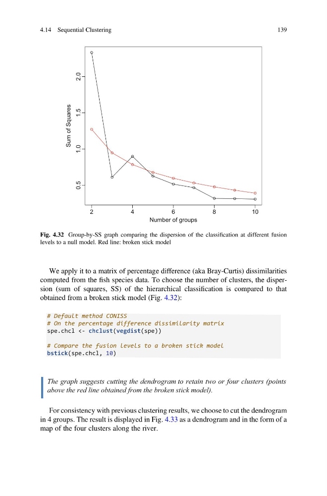
We apply it to a matrix of percentage difference (aka Bray-Curtis) dissimilarities
computed from the fish species data. To choose the number of clusters, the dispersion (sum of squares, SS) of the hierarchical classification is compared to that
obtained from a broken stick model (Fig. 4.32):
# Default method CONISS
# On the percentage difference dissimilarity matrix
spe.chcl <- chclust(vegdist(spe))
# Compare the fusion levels to a broken stick model
bstick(spe.chcl, 10)
The graph suggests cutting the dendrogram to retain two or four clusters (points
above the red line obtained from the broken stick model).
For consistency with previous clustering results, we choose to cut the dendrogram
in 4 groups. The result is displayed in Fig. 4.33 as a dendrogram and in the form of a
map of the four clusters along the river.
2
4
6
8
1 0
0.5
1.0
1.5
2.0
Number of groups
Sum of Squares
Fig. 4.32 Group-by-SS graph comparing the dispersion of the classification at different fusion
levels to a null model. Red line: broken stick model
4.14 Sequential Clustering
139