

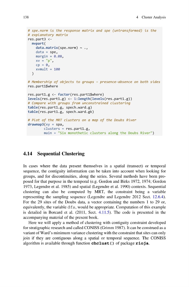
# spe.norm is the response matrix and spe (untransformed) is the
# explanatory matrix
res.part3
data = spe,
margin = 0.08,
xv = "p",
cp = 0,
xvmult = 100
)
# Membership of objects to groups – presence-absence on both sides
res.part1$where
res.part1.g <- factor(res.part1$where)
levels(res.part1.g) <- 1:length(levels(res.part1.g))
# Compare with groups from unconstrained clustering
table(res.part1.g, spech.ward.g)
table(res.part1.g, spech.ward.gk)
# Plot of the MRT clusters on a map of the Doubs River
drawmap3(xy = spa,
clusters = res.part1.g,
main = "Six monothetic clusters along the Doubs River")
4.14 Sequential Clustering
In cases where the data present themselves in a spatial (transect) or temporal
sequence, the contiguity information can be taken into account when looking for
groups, and for discontinuities, along the series. Several methods have been proposed for that purpose in the temporal (e.g. Gordon and Birks 1972, 1974; Gordon
1973, Legendre et al. 1985) and spatial (Legendre et al. 1990) contexts. Sequential
clustering can also be computed by MRT, the constraint being a variable
representing the sampling sequence (Legendre and Legendre 2012 Sect. 12.6.4).
For the 29 sites of the Doubs data, a vector containing the numbers 1 to 29 or,
equivalently, the variable dfs, would be appropriate. Computation of this example
is detailed in Borcard et al. (2011, Sect. 4.11.5). The code is presented in the
accompanying material of the present book.
Here we will apply a method of clustering with contiguity constraint developed
for stratigraphic research and called CONISS (Grimm 1987). It can be construed as a
variant of Ward’s minimum variance clustering with the constraint that sites can only
join if they are contiguous along a spatial or temporal sequence. The CONISS
algorithm is available through function chclust() of package rioja.
138
4 Cluster Analysis
# explanatory matrix
res.part3
data = spe,
margin = 0.08,
xv = "p",
cp = 0,
xvmult = 100
)
# Membership of objects to groups – presence-absence on both sides
res.part1$where
res.part1.g <- factor(res.part1$where)
levels(res.part1.g) <- 1:length(levels(res.part1.g))
# Compare with groups from unconstrained clustering
table(res.part1.g, spech.ward.g)
table(res.part1.g, spech.ward.gk)
# Plot of the MRT clusters on a map of the Doubs River
drawmap3(xy = spa,
clusters = res.part1.g,
main = "Six monothetic clusters along the Doubs River")
4.14 Sequential Clustering
In cases where the data present themselves in a spatial (transect) or temporal
sequence, the contiguity information can be taken into account when looking for
groups, and for discontinuities, along the series. Several methods have been proposed for that purpose in the temporal (e.g. Gordon and Birks 1972, 1974; Gordon
1973, Legendre et al. 1985) and spatial (Legendre et al. 1990) contexts. Sequential
clustering can also be computed by MRT, the constraint being a variable
representing the sampling sequence (Legendre and Legendre 2012 Sect. 12.6.4).
For the 29 sites of the Doubs data, a vector containing the numbers 1 to 29 or,
equivalently, the variable dfs, would be appropriate. Computation of this example
is detailed in Borcard et al. (2011, Sect. 4.11.5). The code is presented in the
accompanying material of the present book.
Here we will apply a method of clustering with contiguity constraint developed
for stratigraphic research and called CONISS (Grimm 1987). It can be construed as a
variant of Ward’s minimum variance clustering with the constraint that sites can only
join if they are contiguous along a spatial or temporal sequence. The CONISS
algorithm is available through function chclust() of package rioja.
138
4 Cluster Analysis