

# spe.pa (presence-absence) is the response and the explanatory
# matrix
par(mfrow = c(1, 2))
spe.pa <- decostand(spe, "pa")
res.part1
data = spe.pa,
margin = 0.08,
xv = "p",
xvmult = 100
)
# spe.norm is the response, spe.pa is the explanatory matrix
res.part2
data = spe.pa,
margin = 0.08,
xv = "p",
xvmult = 100
)
0
50
100
150
20
40
60
80
100
Six monothetic clusters along the Doubs River
x coordinate (km)
y coordinate (km)
Upstream
Downstream
21
3
4
5
6
7
9
10
11
12
13
14
15
16
17
18
19
20
21
22
23
24
25
26
27
28
29
30
Cluster 1
Cluster 2
Cluster 3
Cluster 4
Cluster 5
Cluster 6
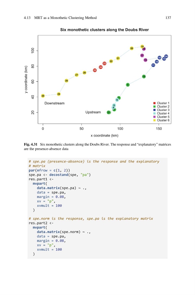
Fig. 4.31 Six monothetic clusters along the Doubs River. The response and “explanatory” matrices
are the presence-absence data
4.13 MRT as a Monothetic Clustering Method
137
# matrix
par(mfrow = c(1, 2))
spe.pa <- decostand(spe, "pa")
res.part1
data = spe.pa,
margin = 0.08,
xv = "p",
xvmult = 100
)
# spe.norm is the response, spe.pa is the explanatory matrix
res.part2
data = spe.pa,
margin = 0.08,
xv = "p",
xvmult = 100
)
0
50
100
150
20
40
60
80
100
Six monothetic clusters along the Doubs River
x coordinate (km)
y coordinate (km)
Upstream
Downstream
21
3
4
5
6
7
9
10
11
12
13
14
15
16
17
18
19
20
21
22
23
24
25
26
27
28
29
30
Cluster 1
Cluster 2
Cluster 3
Cluster 4
Cluster 5
Cluster 6
Fig. 4.31 Six monothetic clusters along the Doubs River. The response and “explanatory” matrices
are the presence-absence data
4.13 MRT as a Monothetic Clustering Method
137