

# For each significant species, find the leaf with the highest
# IndVal
spe.ch.MRT.indval$maxcls[which(pval.adj3 <= 0.05)]
Satr Phph Baba Rham Legi Cyca Abbr Blbj Alal Anan
1
1
4
4
4
4
4
4
4
4
# IndVal value in the best leaf for each significant species
spe.ch.MRT.indval$indcls[which(pval.adj3 <= 0.05)]
Satr
Phph
Baba
Rham
Legi
Cyca
Abbr
0.7899792 0.5422453 0.6547659 0.8743
0.7079525 0.6700303 0.8460903
930 0.6568224 0.7964617 0.9000000
Blbj
Alal
Anan
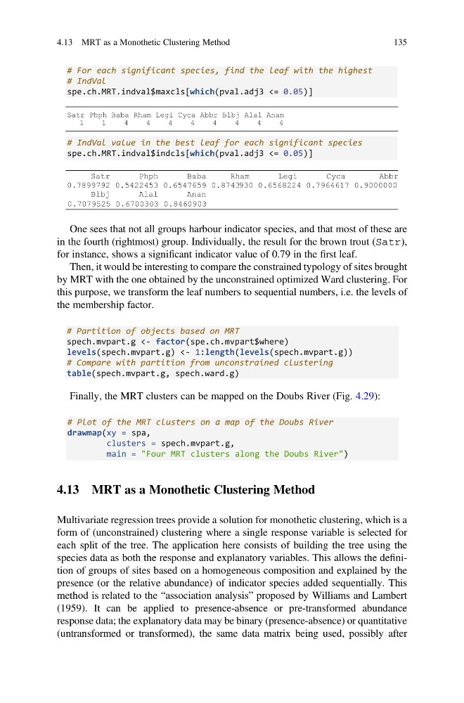
One sees that not all groups harbour indicator species, and that most of these are
in the fourth (rightmost) group. Individually, the result for the brown trout (Satr),
for instance, shows a significant indicator value of 0.79 in the first leaf.
Then, it would be interesting to compare the constrained typology of sites brought
by MRT with the one obtained by the unconstrained optimized Ward clustering. For
this purpose, we transform the leaf numbers to sequential numbers, i.e. the levels of
the membership factor.
# Partition of objects based on MRT
spech.mvpart.g <- factor(spe.ch.mvpart$where)
levels(spech.mvpart.g) <- 1:length(levels(spech.mvpart.g))
# Compare with partition from unconstrained clustering
table(spech.mvpart.g, spech.ward.g)
Finally, the MRT clusters can be mapped on the Doubs River (Fig. 4.29):
# Plot of the MRT clusters on a map of the Doubs River
drawmap(xy = spa,
clusters = spech.mvpart.g,
main = "Four MRT clusters along the Doubs River")
4.13 MRT as a Monothetic Clustering Method
Multivariate regression trees provide a solution for monothetic clustering, which is a
form of (unconstrained) clustering where a single response variable is selected for
each split of the tree. The application here consists of building the tree using the
species data as both the response and explanatory variables. This allows the definition of groups of sites based on a homogeneous composition and explained by the
presence (or the relative abundance) of indicator species added sequentially. This
method is related to the “association analysis” proposed by Williams and Lambert
(1959). It can be applied to presence-absence or pre-transformed abundance
response data; the explanatory data may be binary (presence-absence) or quantitative
(untransformed or transformed), the same data matrix being used, possibly after
4.13 MRT as a Monothetic Clustering Method
135
# IndVal
spe.ch.MRT.indval$maxcls[which(pval.adj3 <= 0.05)]
Satr Phph Baba Rham Legi Cyca Abbr Blbj Alal Anan
1
1
4
4
4
4
4
4
4
4
# IndVal value in the best leaf for each significant species
spe.ch.MRT.indval$indcls[which(pval.adj3 <= 0.05)]
Satr
Phph
Baba
Rham
Legi
Cyca
Abbr
0.7899792 0.5422453 0.6547659 0.8743
0.7079525 0.6700303 0.8460903
930 0.6568224 0.7964617 0.9000000
Blbj
Alal
Anan
One sees that not all groups harbour indicator species, and that most of these are
in the fourth (rightmost) group. Individually, the result for the brown trout (Satr),
for instance, shows a significant indicator value of 0.79 in the first leaf.
Then, it would be interesting to compare the constrained typology of sites brought
by MRT with the one obtained by the unconstrained optimized Ward clustering. For
this purpose, we transform the leaf numbers to sequential numbers, i.e. the levels of
the membership factor.
# Partition of objects based on MRT
spech.mvpart.g <- factor(spe.ch.mvpart$where)
levels(spech.mvpart.g) <- 1:length(levels(spech.mvpart.g))
# Compare with partition from unconstrained clustering
table(spech.mvpart.g, spech.ward.g)
Finally, the MRT clusters can be mapped on the Doubs River (Fig. 4.29):
# Plot of the MRT clusters on a map of the Doubs River
drawmap(xy = spa,
clusters = spech.mvpart.g,
main = "Four MRT clusters along the Doubs River")
4.13 MRT as a Monothetic Clustering Method
Multivariate regression trees provide a solution for monothetic clustering, which is a
form of (unconstrained) clustering where a single response variable is selected for
each split of the tree. The application here consists of building the tree using the
species data as both the response and explanatory variables. This allows the definition of groups of sites based on a homogeneous composition and explained by the
presence (or the relative abundance) of indicator species added sequentially. This
method is related to the “association analysis” proposed by Williams and Lambert
(1959). It can be applied to presence-absence or pre-transformed abundance
response data; the explanatory data may be binary (presence-absence) or quantitative
(untransformed or transformed), the same data matrix being used, possibly after
4.13 MRT as a Monothetic Clustering Method
135