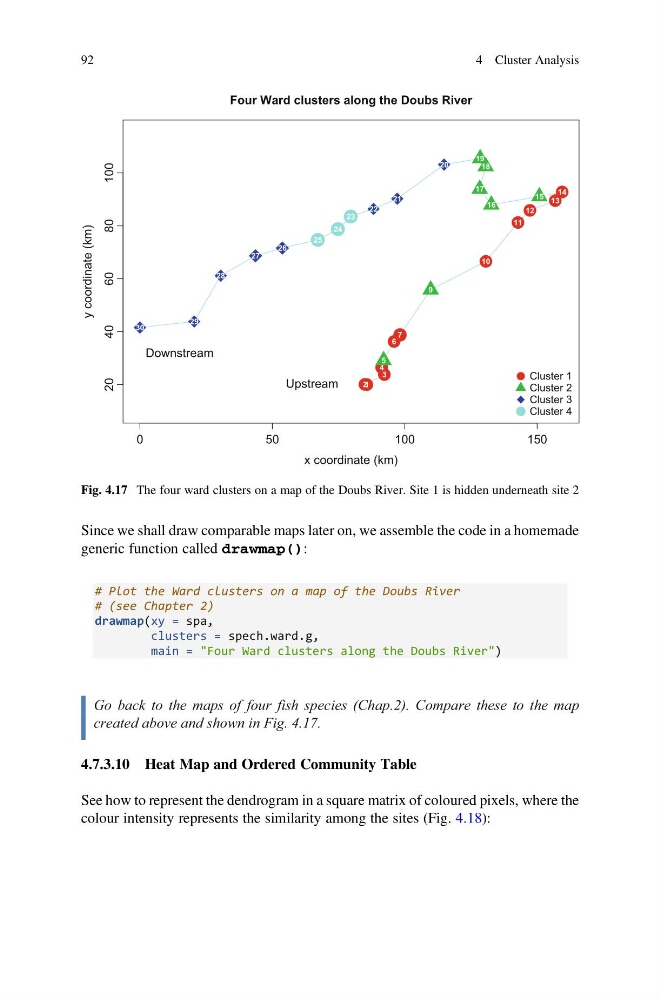
Since we shall draw comparable maps later on, we assemble the code in a homemade
generic function called drawmap():
# Plot the Ward clusters on a map of the Doubs River
# (see Chapter 2)
drawmap(xy = spa,
clusters = spech.ward.g,
main = "Four Ward clusters along the Doubs River")
Go back to the maps of four fish species (Chap.2). Compare these to the map
created above and shown in Fig. 4.17.
4.7.3.10 Heat Map and Ordered Community Table
See how to represent the dendrogram in a square matrix of coloured pixels, where the
colour intensity represents the similarity among the sites (Fig. 4.18):
0
50
100
150
20
40
60
80
100
Four Ward clusters along the Doubs River
x coordinate (km)
y coordinate (km)
Upstream
Downstream
1
2
3
4
5
6
7
9
10
11
12
13
14
15
16
17
18
19
20
21
22
23
24
25
26
27
28
29
30
Cluster 1
Cluster 2
Cluster 3
Cluster 4
Fig. 4.17 The four ward clusters on a map of the Doubs River. Site 1 is hidden underneath site 2
92
4 Cluster Analysis