

179
5000 years ago have almost the same δ
13
C values because the mechanism of carbon
assimilation has remained constant; however, their Δ
14
C values can easily be distinguished. Secondly, the calculation of Δ
14
C by internal correction using δ
13
C values
eliminates any effects from isotope fractionation (Stuiver and Polach 1977). For
these two reasons, it is possible to overcome the above-described problems with the
conventional δ
13
C approach by combining δ
13
C and Δ
14
C measurements.
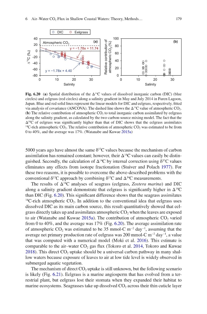
The results of Δ
14
C analyses of seagrass (eelgrass, Zostera marina) and DIC
along a salinity gradient demonstrate that eelgrass is significantly higher in Δ
14
C
than DIC (Fig. 6.20). This significant difference shows that the seagrass assimilates
14
C-rich atmospheric CO 2 . In addition to the conventional idea that eelgrass uses
dissolved DIC as its main carbon source, this result quantitatively showed that eelgrass directly takes up and assimilates atmospheric CO 2 when the leaves are exposed
to air (Watanabe and Kuwae 2015a). The contribution of atmospheric CO 2 varied
from 0 to 40%, and the average was 17% (Fig. 6.20). The average assimilation rate
of atmospheric CO 2 was estimated to be 35 mmol-C m
−2
day
−1
, assuming that the
average net primary production rate of eelgrass was 200 mmol-C m
−2
day
−1
, a value
that was computed with a numerical model (Moki et al. 2016). This estimate is
comparable to the air–water CO 2 gas flux (Tokoro et al. 2014, Tokoro and Kuwae
2018). This direct CO 2 uptake should be a universal carbon pathway in many shallow waters because exposure of leaves to air at low tide level is widely observed in
submerged aquatic vegetation.
The mechanism of direct CO 2 uptake is still unknown, but the following scenario
is likely (Fig. 6.21). Eelgrass is a marine angiosperm that has evolved from a terrestrial plant, but eelgrass lost their stomata when they expanded their habitat to
marine ecosystems. Seagrasses take up dissolved CO 2 across their thin cuticle layer
0
20
40
60
80
100
0
1 0
2 0
3 0
-80
-60
-40
-20
0
20
40
0
1 0
2 0
3 0
∆
14
C (‰)
Salinity
Relative contribution of
atmospheric CO
2 (%)
(a)
Atmospheric CO 2
y = −1.78x + 4.40
y = −1.78x + 11.74
DIC
E elgrass
(b)
Salinity
Fig. 6.20 (a) Spatial distribution of the Δ
14
C values of dissolved inorganic carbon (DIC) (blue
circles) and eelgrass (red circles) along a salinity gradient in May and July 2014 in Furen Lagoon,
Japan. Blue and red solid lines represent the linear models for DIC and eelgrass, respectively, fitted
via analysis of covariance (ANCOVA). The dashed line shows the Δ
14 C value of atmospheric CO 2 .
(b) The relative contribution of atmospheric CO 2 to total inorganic carbon assimilated by eelgrass
along the salinity gradient, as calculated by the two-carbon-source mixing model. The fact that the
Δ
14 C of eelgrass was significantly higher than that of DIC shows that the eelgrass assimilates
14 C-rich atmospheric CO 2 . The relative contribution of atmospheric CO 2 was estimated to be from
0 to 40%, and the average was 17%. (Watanabe and Kuwae 2015a)
6 Air–Water CO 2 Flux in Shallow Coastal Waters: Theory, Methods…
5000 years ago have almost the same δ
13
C values because the mechanism of carbon
assimilation has remained constant; however, their Δ
14
C values can easily be distinguished. Secondly, the calculation of Δ
14
C by internal correction using δ
13
C values
eliminates any effects from isotope fractionation (Stuiver and Polach 1977). For
these two reasons, it is possible to overcome the above-described problems with the
conventional δ
13
C approach by combining δ
13
C and Δ
14
C measurements.
The results of Δ
14
C analyses of seagrass (eelgrass, Zostera marina) and DIC
along a salinity gradient demonstrate that eelgrass is significantly higher in Δ
14
C
than DIC (Fig. 6.20). This significant difference shows that the seagrass assimilates
14
C-rich atmospheric CO 2 . In addition to the conventional idea that eelgrass uses
dissolved DIC as its main carbon source, this result quantitatively showed that eelgrass directly takes up and assimilates atmospheric CO 2 when the leaves are exposed
to air (Watanabe and Kuwae 2015a). The contribution of atmospheric CO 2 varied
from 0 to 40%, and the average was 17% (Fig. 6.20). The average assimilation rate
of atmospheric CO 2 was estimated to be 35 mmol-C m
−2
day
−1
, assuming that the
average net primary production rate of eelgrass was 200 mmol-C m
−2
day
−1
, a value
that was computed with a numerical model (Moki et al. 2016). This estimate is
comparable to the air–water CO 2 gas flux (Tokoro et al. 2014, Tokoro and Kuwae
2018). This direct CO 2 uptake should be a universal carbon pathway in many shallow waters because exposure of leaves to air at low tide level is widely observed in
submerged aquatic vegetation.
The mechanism of direct CO 2 uptake is still unknown, but the following scenario
is likely (Fig. 6.21). Eelgrass is a marine angiosperm that has evolved from a terrestrial plant, but eelgrass lost their stomata when they expanded their habitat to
marine ecosystems. Seagrasses take up dissolved CO 2 across their thin cuticle layer
0
20
40
60
80
100
0
1 0
2 0
3 0
-80
-60
-40
-20
0
20
40
0
1 0
2 0
3 0
∆
14
C (‰)
Salinity
Relative contribution of
atmospheric CO
2 (%)
(a)
Atmospheric CO 2
y = −1.78x + 4.40
y = −1.78x + 11.74
DIC
E elgrass
(b)
Salinity
Fig. 6.20 (a) Spatial distribution of the Δ
14
C values of dissolved inorganic carbon (DIC) (blue
circles) and eelgrass (red circles) along a salinity gradient in May and July 2014 in Furen Lagoon,
Japan. Blue and red solid lines represent the linear models for DIC and eelgrass, respectively, fitted
via analysis of covariance (ANCOVA). The dashed line shows the Δ
14 C value of atmospheric CO 2 .
(b) The relative contribution of atmospheric CO 2 to total inorganic carbon assimilated by eelgrass
along the salinity gradient, as calculated by the two-carbon-source mixing model. The fact that the
Δ
14 C of eelgrass was significantly higher than that of DIC shows that the eelgrass assimilates
14 C-rich atmospheric CO 2 . The relative contribution of atmospheric CO 2 was estimated to be from
0 to 40%, and the average was 17%. (Watanabe and Kuwae 2015a)
6 Air–Water CO 2 Flux in Shallow Coastal Waters: Theory, Methods…