

25. Ecosystem Modeling
system. One important measure is the time constant
(or turnover time )-the time needed for the amount
of material flowing through the compartment at
equilibrium to equal the amount of material in the
compartment. The time constant is often denoted
with T (for an entire system) or Ti (for the loth compartment in a system).
Complexity in a compartment model arises in the
linking together of compartments representing parts
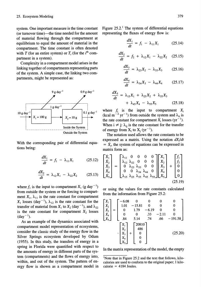
of the system. A simple case, the linking two compartments, might be represented as:
9 gday-l
0.9 g day-l
With the corresponding pair of differential equations being:
(25.12)
(25.13)
where II is the input to compartment XI (g day-I)
from outside the system or the forcing to compartment Xl> Al1 is the rate constant for compartment
XI losses (day-I), A12 is the rate constant for the
transfer of material from XI to X 2 (day-I), and A22
is the rate constant for compartment X2 losses
(day-I).
As an example of the dynamics associated with
compartment model representation of ecosystems,
consider the classic study of the energy flow in the
Silver Springs ecosystem developed by Odum
(1955). In this study, the transfers of energy in a
spring in Florida were quantified with respect to
the amounts of energy in different parts of the system (compartments) and the flows of energy into,
within, and out of the system. The pattern of energy flow is shown as a compartment model in
379
Figure 25.2.1 The system of differential equations
representing the fluxes of energy flow is:
dXI
- = II - Al1 XI
dt
dX 2
dt = 12 + A12 X I - A22X2
dX3
A23 X2
A33 X3
=
dt
dX4
A34X3 - A44X4
dt
d!s = AISXI + A2S X2 + A3S X3
+ A4S X4 - ASSXS
(25.14)
(25.15)
(25.16)
(25.17)
(25.18)
where fi is the input to compartment Xi
(kcal m - 2 yr - I) from outside the system and Aii is
the rate constant for compartment Xi losses (yr- I ).
When i "'" j: Aij is the rate constant for the transfer
of energy from Xi to Xj (yr- I ).
The notation used allows the rate constants to be
expressed as a matrix. Using the notation dX/dt
= Xi' the system of equations can be expressed in
matrix form as:
or using the values for rate constants calculated
from the information from Figure 25.2:
[ ~:] [~~~8 -1~.81 ~
X3 =
0
1.79 -6.19
X4
0
0
.33
Xs
.84
5.14
.74
[ i:] [2~:!O]
. X3 +
0
X4
0
Xs
0
o
o
o
-2.11
.66
jJ
(25.20)
In the matrix representation of the model, the empty
lNote that in Figure 25.2 and the text that follows, kilocalories are used to conform to the original paper; 1 kilocalorie = 4184 Joules.
system. One important measure is the time constant
(or turnover time )-the time needed for the amount
of material flowing through the compartment at
equilibrium to equal the amount of material in the
compartment. The time constant is often denoted
with T (for an entire system) or Ti (for the loth compartment in a system).
Complexity in a compartment model arises in the
linking together of compartments representing parts
of the system. A simple case, the linking two compartments, might be represented as:
9 gday-l
0.9 g day-l
With the corresponding pair of differential equations being:
(25.12)
(25.13)
where II is the input to compartment XI (g day-I)
from outside the system or the forcing to compartment Xl> Al1 is the rate constant for compartment
XI losses (day-I), A12 is the rate constant for the
transfer of material from XI to X 2 (day-I), and A22
is the rate constant for compartment X2 losses
(day-I).
As an example of the dynamics associated with
compartment model representation of ecosystems,
consider the classic study of the energy flow in the
Silver Springs ecosystem developed by Odum
(1955). In this study, the transfers of energy in a
spring in Florida were quantified with respect to
the amounts of energy in different parts of the system (compartments) and the flows of energy into,
within, and out of the system. The pattern of energy flow is shown as a compartment model in
379
Figure 25.2.1 The system of differential equations
representing the fluxes of energy flow is:
dXI
- = II - Al1 XI
dt
dX 2
dt = 12 + A12 X I - A22X2
dX3
A23 X2
A33 X3
=
dt
dX4
A34X3 - A44X4
dt
d!s = AISXI + A2S X2 + A3S X3
+ A4S X4 - ASSXS
(25.14)
(25.15)
(25.16)
(25.17)
(25.18)
where fi is the input to compartment Xi
(kcal m - 2 yr - I) from outside the system and Aii is
the rate constant for compartment Xi losses (yr- I ).
When i "'" j: Aij is the rate constant for the transfer
of energy from Xi to Xj (yr- I ).
The notation used allows the rate constants to be
expressed as a matrix. Using the notation dX/dt
= Xi' the system of equations can be expressed in
matrix form as:
or using the values for rate constants calculated
from the information from Figure 25.2:
[ ~:] [~~~8 -1~.81 ~
X3 =
0
1.79 -6.19
X4
0
0
.33
Xs
.84
5.14
.74
[ i:] [2~:!O]
. X3 +
0
X4
0
Xs
0
o
o
o
-2.11
.66
jJ
(25.20)
In the matrix representation of the model, the empty
lNote that in Figure 25.2 and the text that follows, kilocalories are used to conform to the original paper; 1 kilocalorie = 4184 Joules.