

378
procedures that amount to assuming that the materials going in and out of a compartment are equal.
This is true when the amount of material in the
compartment is constant. In other cases, fluxes are
measured by assuming that rates of transfer noted
in laboratory experiments or in small field experiments and applied to larger systems.
The formulation of element cycling compartment diagrams (or models) involves subtle, underlying assumptions about the constancy of ecosystems and the extrapolation of observations to larger
spatial scales. For these reasons, ecosystems, such
as watersheds, in which some of the fluxes can be
measured directly have great scientific importance
(Bormann and Likens 1979).
Fonnulation of Compartment Models
for Ecosystem Studies
The usual application of compartment models in
ecology involves the internal and external transfers
of nutrients and energy in ecosystems. A straightforward introduction to these models is through the
terms and procedures associated with estimating
the parameters of the model. The fundamental unit
of a compartment model is the single compartment
and the associated flows of material or energy in
and out of the compartment:
Outside the System
I
I
I
Inside the System
I
I
I
flUX 1N
: flux OUT
I
I
•
I
I
I
I
I
I
I
I
g day-I
XI = 100g
I
10 g day
I
10
-I
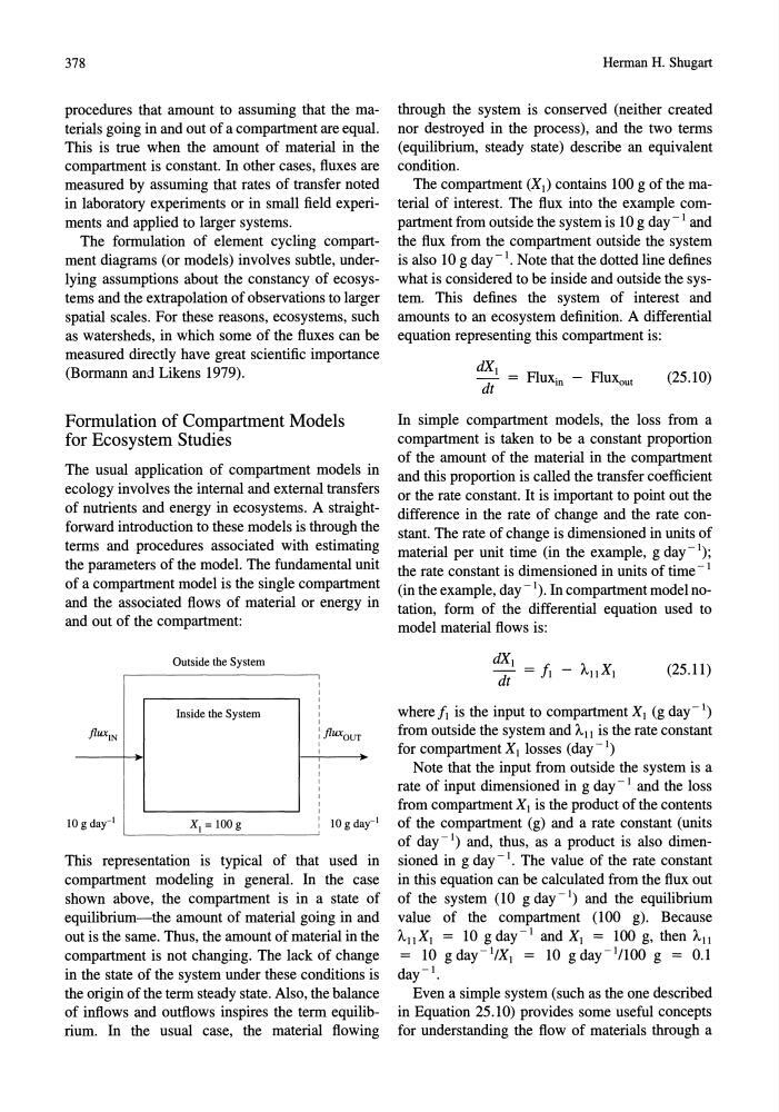
This representation is typical of that used in
compartment modeling in general. In the case
shown above, the compartment is in a state of
equilibrium-the amount of material going in and
out is the same. Thus, the amount of material in the
compartment is not changing. The lack of change
in the state of the system under these conditions is
the origin of the term steady state. Also, the balance
of inflows and outflows inspires the term equilibrium. In the usual case, the material flowing
Herman H. Shugart
through the system is conserved (neither created
nor destroyed in the process), and the two terms
(equilibrium, steady state) describe an equivalent
condition.
The compartment (XI) contains 100 g of the material of interest. The flux into the example compartment from outside the system is 109 day - I and
the flux from the compartment outside the system
is also 10 g day -I. Note that the dotted line defines
what is considered to be inside and outside the system. This defines the system of interest and
amounts to an ecosystem definition. A differential
equation representing this compartment is:
dX I
- = FlUXin - Fluxout
dt
(25.10)
In simple compartment models, the loss from a
compartment is taken to be a constant proportion
of the amount of the material in the compartment
and this proportion is called the transfer coefficient
or the rate constant. It is important to point out the
difference in the rate of change and the rate constant. The rate of change is dimensioned in units of
material per unit time (in the example, g day-I);
the rate constant is dimensioned in units of time - I
(in the example, day-I). In compartment model notation, form of the differential equation used to
model material flows is:
(25.11)
where II is the input to compartment XI (g day-I)
from outside the system and All is the rate constant
for compartment XI losses (day - I)
Note that the input from outside the system is a
rate of input dimensioned in g day - I and the loss
from compartment XI is the product of the contents
of the compartment (g) and a rate constant (units
of day - I) and, thus, as a product is also dimensioned in g day - I. The value of the rate constant
in this equation can be calculated from the flux out
of the system (10 g day-I) and the equilibrium
value of the compartment (100 g). Because
A11XI = 10 g day-I and XI = 100 g, then All
= 10 g day-I/X I = 10 g day- 1 /100 g = 0.1
day-I.
Even a simple system (such as the one described
in Equation 25.10) provides some useful concepts
for understanding the flow of materials through a
procedures that amount to assuming that the materials going in and out of a compartment are equal.
This is true when the amount of material in the
compartment is constant. In other cases, fluxes are
measured by assuming that rates of transfer noted
in laboratory experiments or in small field experiments and applied to larger systems.
The formulation of element cycling compartment diagrams (or models) involves subtle, underlying assumptions about the constancy of ecosystems and the extrapolation of observations to larger
spatial scales. For these reasons, ecosystems, such
as watersheds, in which some of the fluxes can be
measured directly have great scientific importance
(Bormann and Likens 1979).
Fonnulation of Compartment Models
for Ecosystem Studies
The usual application of compartment models in
ecology involves the internal and external transfers
of nutrients and energy in ecosystems. A straightforward introduction to these models is through the
terms and procedures associated with estimating
the parameters of the model. The fundamental unit
of a compartment model is the single compartment
and the associated flows of material or energy in
and out of the compartment:
Outside the System
I
I
I
Inside the System
I
I
I
flUX 1N
: flux OUT
I
I
•
I
I
I
I
I
I
I
I
g day-I
XI = 100g
I
10 g day
I
10
-I
This representation is typical of that used in
compartment modeling in general. In the case
shown above, the compartment is in a state of
equilibrium-the amount of material going in and
out is the same. Thus, the amount of material in the
compartment is not changing. The lack of change
in the state of the system under these conditions is
the origin of the term steady state. Also, the balance
of inflows and outflows inspires the term equilibrium. In the usual case, the material flowing
Herman H. Shugart
through the system is conserved (neither created
nor destroyed in the process), and the two terms
(equilibrium, steady state) describe an equivalent
condition.
The compartment (XI) contains 100 g of the material of interest. The flux into the example compartment from outside the system is 109 day - I and
the flux from the compartment outside the system
is also 10 g day -I. Note that the dotted line defines
what is considered to be inside and outside the system. This defines the system of interest and
amounts to an ecosystem definition. A differential
equation representing this compartment is:
dX I
- = FlUXin - Fluxout
dt
(25.10)
In simple compartment models, the loss from a
compartment is taken to be a constant proportion
of the amount of the material in the compartment
and this proportion is called the transfer coefficient
or the rate constant. It is important to point out the
difference in the rate of change and the rate constant. The rate of change is dimensioned in units of
material per unit time (in the example, g day-I);
the rate constant is dimensioned in units of time - I
(in the example, day-I). In compartment model notation, form of the differential equation used to
model material flows is:
(25.11)
where II is the input to compartment XI (g day-I)
from outside the system and All is the rate constant
for compartment XI losses (day - I)
Note that the input from outside the system is a
rate of input dimensioned in g day - I and the loss
from compartment XI is the product of the contents
of the compartment (g) and a rate constant (units
of day - I) and, thus, as a product is also dimensioned in g day - I. The value of the rate constant
in this equation can be calculated from the flux out
of the system (10 g day-I) and the equilibrium
value of the compartment (100 g). Because
A11XI = 10 g day-I and XI = 100 g, then All
= 10 g day-I/X I = 10 g day- 1 /100 g = 0.1
day-I.
Even a simple system (such as the one described
in Equation 25.10) provides some useful concepts
for understanding the flow of materials through a