

Modern Clustering Techniques and A. Vatova's Community Classification
273
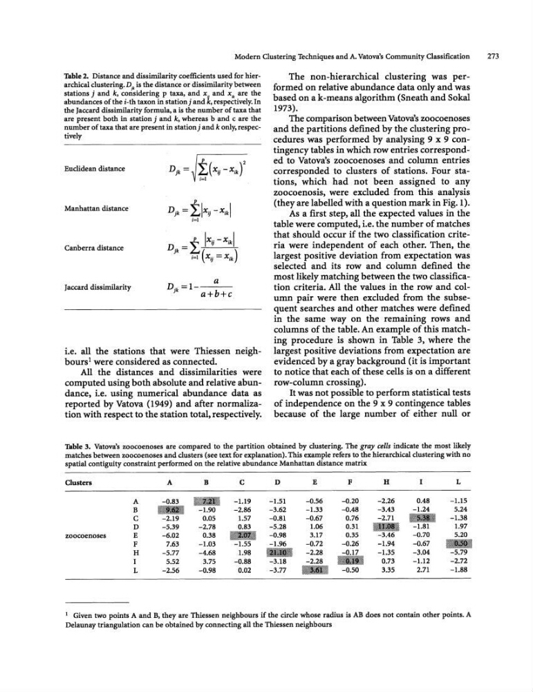
Table 2. Distance and dissimilarity coefficients used for hierarchical clustering. Djt is the distance or dissimilarity between
stations j and k, considering p taxa, and x .. and xii< are the
abundances of the i-th taxon in station j and k, respectively. In
the Jaccard dissimilarity formula, a is the number of taxa that
are present both in station j and k, whereas band c are the
number of taxa that are present in station j and k only, respectively
Euclidean distance
Manhattan distance
Canberra distance
Jaccard dissimilarity
a
D· k = 1 - - - -
1
a+b+c
i.e. all the stations that were Thiessen neighbours! were considered as connected.
All the distances and dissimilarities were
computed using both absolute and relative abundance, i.e. using numerical abundance data as
reported by Vatova (1949) and after normalization with respect to the station total, respectively.
The non-hierarchical clustering was performed on relative abundance data only and was
based on a k-means algorithm (Sneath and Sokal
1973).
The comparison between Vatova's zoocoenoses
and the partitions deflned by the clustering procedures was performed by analysing 9 x 9 contingency tables in which row entries corresponded to Vatow's zoocoenoses and column entries
corresponded to clusters of stations. Four stations, which had not been assigned to any
zoocoenosis, were excluded from this analysis
(they are labelled with a question mark in Fig.I).
As a flrst step. all the expected values in the
table were computed, i.e. the number of matches
that should occur if the two classiflcation criteria were independent of each other. Then, the
largest positive deviation from expectation was
selected and its row and column deflned the
most likely matching between the two classification criteria. All the values in the row and column pair were then excluded from the subsequent searches and other matches were deflned
in the same way on the remaining rows and
columns of the table. An example of this matching procedure is shown in Table 3, where the
largest positive deviations from expectation are
evidenced by a gray background (it is important
to notice that each of these cells is on a different
row-column crossing).
It was not possible to perform statistical tests
of independence on the 9 x 9 contingence tables
because of the large number of either null or
Table 3. Vatova's zoocoenoses are compared to the partition obtained by clustering. The gray cells indicate the most likely
matches between zoocoenoses and clusters (see text for explanation). This example refers to the hierarchical clustering with no
spatial contiguity constraint performed on the relative abundance Manhattan distance matrix
Clusters
A
B
C
D
E
F
H
L
A
-1.19
-1.51
-0.56
-0.20
-2.26
0.48
-1.15
B
-2.86
-3.62
-1.33
-0.48
-3.43
5.24
C
0.05
1.57
-0.81
-0.67
0.76
-2.71
-1.38
D
-5.39
-2.78
0.83
-5.28
1.06
0.31
1.97
zoocoenoses
E
-6.02
0.38
-0.98
3.17
0.35
-0.70
5.20
F
7.63
-1.03
-0.72
-0.26
-1.94
-0.67
H
-5.77
-4.68
1.98
-2.28
-1.35
-3.04
I
5.52
3.75
-0.88
0.73
-1.12
-2.72
L
-2.56
-0.98
0.02
-3.77
-0.50
3.35
2.71
-1.88
I Given two points A and B, they are Thiessen neighbours if the circle whose radius is AB does not contain other points. A
De1aunay triangulation can be obtained by connecting all the Thiessen neighbours
273
Table 2. Distance and dissimilarity coefficients used for hierarchical clustering. Djt is the distance or dissimilarity between
stations j and k, considering p taxa, and x .. and xii< are the
abundances of the i-th taxon in station j and k, respectively. In
the Jaccard dissimilarity formula, a is the number of taxa that
are present both in station j and k, whereas band c are the
number of taxa that are present in station j and k only, respectively
Euclidean distance
Manhattan distance
Canberra distance
Jaccard dissimilarity
a
D· k = 1 - - - -
1
a+b+c
i.e. all the stations that were Thiessen neighbours! were considered as connected.
All the distances and dissimilarities were
computed using both absolute and relative abundance, i.e. using numerical abundance data as
reported by Vatova (1949) and after normalization with respect to the station total, respectively.
The non-hierarchical clustering was performed on relative abundance data only and was
based on a k-means algorithm (Sneath and Sokal
1973).
The comparison between Vatova's zoocoenoses
and the partitions deflned by the clustering procedures was performed by analysing 9 x 9 contingency tables in which row entries corresponded to Vatow's zoocoenoses and column entries
corresponded to clusters of stations. Four stations, which had not been assigned to any
zoocoenosis, were excluded from this analysis
(they are labelled with a question mark in Fig.I).
As a flrst step. all the expected values in the
table were computed, i.e. the number of matches
that should occur if the two classiflcation criteria were independent of each other. Then, the
largest positive deviation from expectation was
selected and its row and column deflned the
most likely matching between the two classification criteria. All the values in the row and column pair were then excluded from the subsequent searches and other matches were deflned
in the same way on the remaining rows and
columns of the table. An example of this matching procedure is shown in Table 3, where the
largest positive deviations from expectation are
evidenced by a gray background (it is important
to notice that each of these cells is on a different
row-column crossing).
It was not possible to perform statistical tests
of independence on the 9 x 9 contingence tables
because of the large number of either null or
Table 3. Vatova's zoocoenoses are compared to the partition obtained by clustering. The gray cells indicate the most likely
matches between zoocoenoses and clusters (see text for explanation). This example refers to the hierarchical clustering with no
spatial contiguity constraint performed on the relative abundance Manhattan distance matrix
Clusters
A
B
C
D
E
F
H
L
A
-1.19
-1.51
-0.56
-0.20
-2.26
0.48
-1.15
B
-2.86
-3.62
-1.33
-0.48
-3.43
5.24
C
0.05
1.57
-0.81
-0.67
0.76
-2.71
-1.38
D
-5.39
-2.78
0.83
-5.28
1.06
0.31
1.97
zoocoenoses
E
-6.02
0.38
-0.98
3.17
0.35
-0.70
5.20
F
7.63
-1.03
-0.72
-0.26
-1.94
-0.67
H
-5.77
-4.68
1.98
-2.28
-1.35
-3.04
I
5.52
3.75
-0.88
0.73
-1.12
-2.72
L
-2.56
-0.98
0.02
-3.77
-0.50
3.35
2.71
-1.88
I Given two points A and B, they are Thiessen neighbours if the circle whose radius is AB does not contain other points. A
De1aunay triangulation can be obtained by connecting all the Thiessen neighbours