

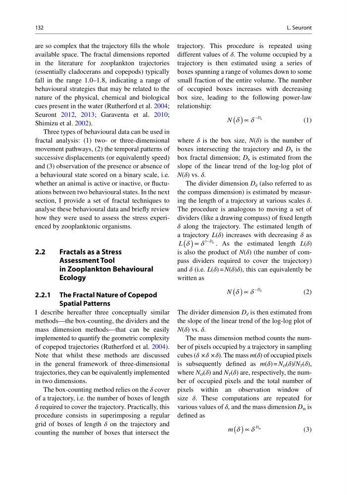
132
are so complex that the trajectory fills the whole
available space. The fractal dimensions reported
in the literature for zooplankton trajectories
(essentially cladocerans and copepods) typically
fall in the range 1.0–1.8, indicating a range of
behavioural strategies that may be related to the
nature of the physical, chemical and biological
cues present in the water (Rutherford et al. 2004;
Seuront 2012, 2013; Garaventa et al. 2010;
Shimizu et al. 2002).
Three types of behavioural data can be used in
fractal analysis: (1) two- or three-dimensional
movement pathways, (2) the temporal patterns of
successive displacements (or equivalently speed)
and (3) observation of the presence or absence of
a behavioural state scored on a binary scale, i.e.
whether an animal is active or inactive, or fluctuations between two behavioural states. In the next
section, I provide a set of fractal techniques to
analyse these behavioural data and briefly review
how they were used to assess the stress experienced by zooplanktonic organisms.
2.2
Fractals as a Stress
Assessment Tool
in Zooplankton Behavioural
Ecology
2.2.1 The Fractal Nature of Copepod
Spatial Patterns
I describe hereafter three conceptually similar
methods—the box-counting, the dividers and the
mass dimension methods—that can be easily
implemented to quantify the geometric complexity
of copepod trajectories (Rutherford et al. 2004).
Note that whilst these methods are discussed
in the general framework of three- dimensional
trajectories, they can be equivalently implemented
in two dimensions.
The box-counting method relies on the δ cover
of a trajectory, i.e. the number of boxes of length
δ required to cover the trajectory. Practically, this
procedure consists in superimposing a regular
grid of boxes of length δ on the trajectory and
counting the number of boxes that intersect the
trajectory. This procedure is repeated using
different values of δ. The volume occupied by a
trajectory is then estimated using a series of
boxes spanning a range of volumes down to some
small fraction of the entire volume. The number
of occupied boxes increases with decreasing
box size, leading to the following power-law
relationship:
N
D b
δ
δ
( )∝
−
(1)
where δ is the box size, N(δ) is the number of
boxes intersecting the trajectory and D b is the
box fractal dimension; D b is estimated from the
slope of the linear trend of the log-log plot of
N(δ) vs. δ.
The divider dimension D d (also referred to as
the compass dimension) is estimated by measuring the length of a trajectory at various scales δ.
The procedure is analogous to moving a set of
dividers (like a drawing compass) of fixed length
δ along the trajectory. The estimated length of
a trajectory L(δ) increases with decreasing δ as
L
D
δ
δ
( )∝
−
1 d
. As the estimated length L(δ)
is also the product of N(δ) (the number of compass dividers required to cover the trajectory)
and δ (i.e. L(δ) = N(δ)δ), this can equivalently be
written as
N
D
δ
δ
( )∝
− d
(2)
The divider dimension D d is then estimated from
the slope of the linear trend of the log-log plot of
N(δ) vs. δ.
The mass dimension method counts the number of pixels occupied by a trajectory in sampling
cubes (δ × δ × δ). The mass m(δ) of occupied pixels
is subsequently defined as m(δ) = N O (δ)/N T (δ),
where N O (δ) and N T (δ) are, respectively, the number of occupied pixels and the total number of
pixels within an observation window of
size δ. These computations are repeated for
various values of δ, and the mass dimension D m is
defined as
m
D
δ
δ
( )∝
m
(3)
L. Seuront
are so complex that the trajectory fills the whole
available space. The fractal dimensions reported
in the literature for zooplankton trajectories
(essentially cladocerans and copepods) typically
fall in the range 1.0–1.8, indicating a range of
behavioural strategies that may be related to the
nature of the physical, chemical and biological
cues present in the water (Rutherford et al. 2004;
Seuront 2012, 2013; Garaventa et al. 2010;
Shimizu et al. 2002).
Three types of behavioural data can be used in
fractal analysis: (1) two- or three-dimensional
movement pathways, (2) the temporal patterns of
successive displacements (or equivalently speed)
and (3) observation of the presence or absence of
a behavioural state scored on a binary scale, i.e.
whether an animal is active or inactive, or fluctuations between two behavioural states. In the next
section, I provide a set of fractal techniques to
analyse these behavioural data and briefly review
how they were used to assess the stress experienced by zooplanktonic organisms.
2.2
Fractals as a Stress
Assessment Tool
in Zooplankton Behavioural
Ecology
2.2.1 The Fractal Nature of Copepod
Spatial Patterns
I describe hereafter three conceptually similar
methods—the box-counting, the dividers and the
mass dimension methods—that can be easily
implemented to quantify the geometric complexity
of copepod trajectories (Rutherford et al. 2004).
Note that whilst these methods are discussed
in the general framework of three- dimensional
trajectories, they can be equivalently implemented
in two dimensions.
The box-counting method relies on the δ cover
of a trajectory, i.e. the number of boxes of length
δ required to cover the trajectory. Practically, this
procedure consists in superimposing a regular
grid of boxes of length δ on the trajectory and
counting the number of boxes that intersect the
trajectory. This procedure is repeated using
different values of δ. The volume occupied by a
trajectory is then estimated using a series of
boxes spanning a range of volumes down to some
small fraction of the entire volume. The number
of occupied boxes increases with decreasing
box size, leading to the following power-law
relationship:
N
D b
δ
δ
( )∝
−
(1)
where δ is the box size, N(δ) is the number of
boxes intersecting the trajectory and D b is the
box fractal dimension; D b is estimated from the
slope of the linear trend of the log-log plot of
N(δ) vs. δ.
The divider dimension D d (also referred to as
the compass dimension) is estimated by measuring the length of a trajectory at various scales δ.
The procedure is analogous to moving a set of
dividers (like a drawing compass) of fixed length
δ along the trajectory. The estimated length of
a trajectory L(δ) increases with decreasing δ as
L
D
δ
δ
( )∝
−
1 d
. As the estimated length L(δ)
is also the product of N(δ) (the number of compass dividers required to cover the trajectory)
and δ (i.e. L(δ) = N(δ)δ), this can equivalently be
written as
N
D
δ
δ
( )∝
− d
(2)
The divider dimension D d is then estimated from
the slope of the linear trend of the log-log plot of
N(δ) vs. δ.
The mass dimension method counts the number of pixels occupied by a trajectory in sampling
cubes (δ × δ × δ). The mass m(δ) of occupied pixels
is subsequently defined as m(δ) = N O (δ)/N T (δ),
where N O (δ) and N T (δ) are, respectively, the number of occupied pixels and the total number of
pixels within an observation window of
size δ. These computations are repeated for
various values of δ, and the mass dimension D m is
defined as
m
D
δ
δ
( )∝
m
(3)
L. Seuront