

Oscillations can occur in simple first-order differential equations provided they are
nonlinear and contain lags. Let us define the differential equation that guides the
change in population size as
ΔN ¼ R Ã LAG N Ã 1 À LAG N
ð
Þ
ð 4:7Þ
with
LAG N ¼ DELAY N; 1
ð
Þ
ð4:8Þ
where DELAY is the built-in function that generates a delayed value of its argument—in our case the state variable N—over a set time frame—in our case 1 full
time period.
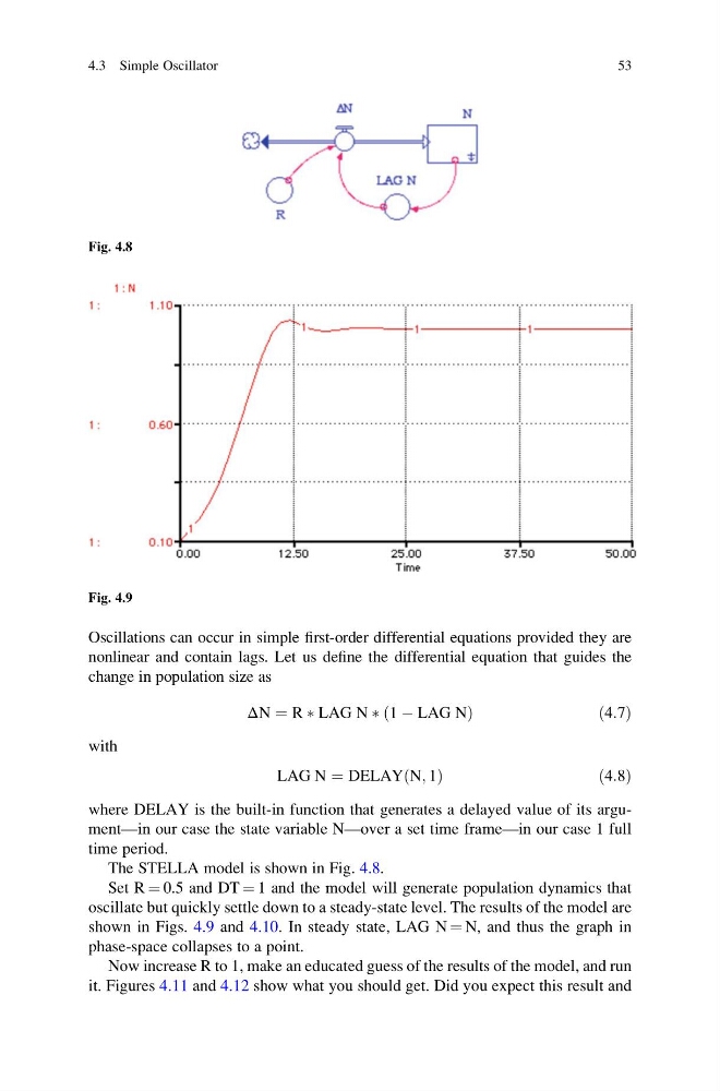
The STELLA model is shown in Fig. 4.8.
Set R ¼ 0.5 and DT ¼ 1 and the model will generate population dynamics that
oscillate but quickly settle down to a steady-state level. The results of the model are
shown in Figs. 4.9 and 4.10. In steady state, LAG N ¼ N, and thus the graph in
phase-space collapses to a point.
Now increase R to 1, make an educated guess of the results of the model, and run
it. Figures 4.11 and 4.12 show what you should get. Did you expect this result and
Fig. 4.8
Fig. 4.9
4.3 Simple Oscillator
53
nonlinear and contain lags. Let us define the differential equation that guides the
change in population size as
ΔN ¼ R Ã LAG N Ã 1 À LAG N
ð
Þ
ð 4:7Þ
with
LAG N ¼ DELAY N; 1
ð
Þ
ð4:8Þ
where DELAY is the built-in function that generates a delayed value of its argument—in our case the state variable N—over a set time frame—in our case 1 full
time period.
The STELLA model is shown in Fig. 4.8.
Set R ¼ 0.5 and DT ¼ 1 and the model will generate population dynamics that
oscillate but quickly settle down to a steady-state level. The results of the model are
shown in Figs. 4.9 and 4.10. In steady state, LAG N ¼ N, and thus the graph in
phase-space collapses to a point.
Now increase R to 1, make an educated guess of the results of the model, and run
it. Figures 4.11 and 4.12 show what you should get. Did you expect this result and
Fig. 4.8
Fig. 4.9
4.3 Simple Oscillator
53