

advantage is such a result to these systems? Kaufman [2], among others, has
proposed that all systems seem to evolve toward higher and higher efficiencies of
operation. Many systems are so highly disturbed by variations in their environment
that their efficiencies are not ever very high. However, if these disturbances can be
held to a minimum, then the evolution of the system becomes more complete, more
efficient but closer to the border of chaotic behavior. Earthquakes and avalanches are
examples of energy storing systems that continuously redistribute the incoming
stresses more and more efficiently until a breaking point is reached and the border
to chaos is opened. Does this mean that the brain and the heart have somehow evolved
close to some maximum efficiency for such organisms? We don’t know the answer to
this question. We do know that the scale of measurement here matters. For example,
if we were to watch the pattern on a patch of natural forest over many centuries, we
would see the rise and sharp fall of the biomass levels, unpredictably. Forest fires and
insects find ample hosts in such forest patches once they have developed a large
amount of dry biomass bound up in relatively few species. The patch evolves or
succeeds to greater and greater efficiency of light energy conversion by getting larger
and fewer species. But the patch also becomes more vulnerable to fire and pests, and
eventually collapses. Yet if we look at the total biomass on a large collection of such
biomasses, whose collapses are not synchronized, this total biomass remains relatively constant. Thus chaotic-like behavior in the small is not seen in the large. Could
this mean that natural systems have “found” chaos in their search for greater
efficiencies and have “learned” to stagger the chaotic events, allowing faster rebound
and large-scale stability? We don’t know the answers here either, but we think
the implications are fascinating. We will return to these questions with our models
on self-organization and catastrophe, presented in Part VII of this book.
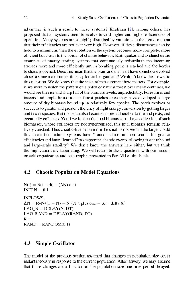
4.2 Chaotic Population Model Equations
N(t) ¼ N(t À dt) + (ΔN) * dt
INIT N ¼ 0.1
INFLOWS:
ΔN ¼ R * N * (1 À N) À N {X_t plus one À X ¼ delta X}
LAG_N ¼ DELAY(N, DT)
LAG_RAND ¼ DELAY(RAND, DT)
R ¼ 1
RAND ¼ RANDOM(0,1)
4.3 Simple Oscillator
The model of the previous section assumed that changes in population size occur
instantaneously in response to the current population. Alternatively, we may assume
that those changes are a function of the population size one time period delayed.
52
4 Steady State, Oscillation, and Chaos in Population Dynamics
proposed that all systems seem to evolve toward higher and higher efficiencies of
operation. Many systems are so highly disturbed by variations in their environment
that their efficiencies are not ever very high. However, if these disturbances can be
held to a minimum, then the evolution of the system becomes more complete, more
efficient but closer to the border of chaotic behavior. Earthquakes and avalanches are
examples of energy storing systems that continuously redistribute the incoming
stresses more and more efficiently until a breaking point is reached and the border
to chaos is opened. Does this mean that the brain and the heart have somehow evolved
close to some maximum efficiency for such organisms? We don’t know the answer to
this question. We do know that the scale of measurement here matters. For example,
if we were to watch the pattern on a patch of natural forest over many centuries, we
would see the rise and sharp fall of the biomass levels, unpredictably. Forest fires and
insects find ample hosts in such forest patches once they have developed a large
amount of dry biomass bound up in relatively few species. The patch evolves or
succeeds to greater and greater efficiency of light energy conversion by getting larger
and fewer species. But the patch also becomes more vulnerable to fire and pests, and
eventually collapses. Yet if we look at the total biomass on a large collection of such
biomasses, whose collapses are not synchronized, this total biomass remains relatively constant. Thus chaotic-like behavior in the small is not seen in the large. Could
this mean that natural systems have “found” chaos in their search for greater
efficiencies and have “learned” to stagger the chaotic events, allowing faster rebound
and large-scale stability? We don’t know the answers here either, but we think
the implications are fascinating. We will return to these questions with our models
on self-organization and catastrophe, presented in Part VII of this book.
4.2 Chaotic Population Model Equations
N(t) ¼ N(t À dt) + (ΔN) * dt
INIT N ¼ 0.1
INFLOWS:
ΔN ¼ R * N * (1 À N) À N {X_t plus one À X ¼ delta X}
LAG_N ¼ DELAY(N, DT)
LAG_RAND ¼ DELAY(RAND, DT)
R ¼ 1
RAND ¼ RANDOM(0,1)
4.3 Simple Oscillator
The model of the previous section assumed that changes in population size occur
instantaneously in response to the current population. Alternatively, we may assume
that those changes are a function of the population size one time period delayed.
52
4 Steady State, Oscillation, and Chaos in Population Dynamics