

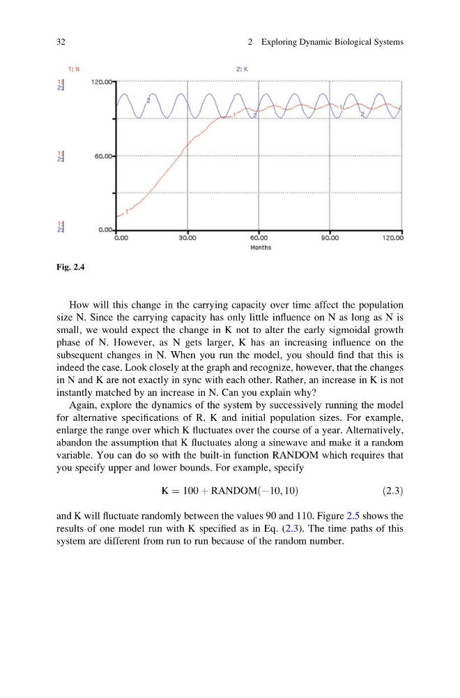
How will this change in the carrying capacity over time affect the population
size N. Since the carrying capacity has only little influence on N as long as N is
small, we would expect the change in K not to alter the early sigmoidal growth
phase of N. However, as N gets larger, K has an increasing influence on the
subsequent changes in N. When you run the model, you should find that this is
indeed the case. Look closely at the graph and recognize, however, that the changes
in N and K are not exactly in sync with each other. Rather, an increase in K is not
instantly matched by an increase in N. Can you explain why?
Again, explore the dynamics of the system by successively running the model
for alternative specifications of R, K and initial population sizes. For example,
enlarge the range over which K fluctuates over the course of a year. Alternatively,
abandon the assumption that K fluctuates along a sinewave and make it a random
variable. You can do so with the built-in function RANDOM which requires that
you specify upper and lower bounds. For example, specify
K ¼ 100 þ RANDOM À10, 10
ð
Þ
ð 2:3Þ
and K will fluctuate randomly between the values 90 and 110. Figure 2.5 shows the
results of one model run with K specified as in Eq. (2.3). The time paths of this
system are different from run to run because of the random number.
Fig. 2.4
32
2 Exploring Dynamic Biological Systems
size N. Since the carrying capacity has only little influence on N as long as N is
small, we would expect the change in K not to alter the early sigmoidal growth
phase of N. However, as N gets larger, K has an increasing influence on the
subsequent changes in N. When you run the model, you should find that this is
indeed the case. Look closely at the graph and recognize, however, that the changes
in N and K are not exactly in sync with each other. Rather, an increase in K is not
instantly matched by an increase in N. Can you explain why?
Again, explore the dynamics of the system by successively running the model
for alternative specifications of R, K and initial population sizes. For example,
enlarge the range over which K fluctuates over the course of a year. Alternatively,
abandon the assumption that K fluctuates along a sinewave and make it a random
variable. You can do so with the built-in function RANDOM which requires that
you specify upper and lower bounds. For example, specify
K ¼ 100 þ RANDOM À10, 10
ð
Þ
ð 2:3Þ
and K will fluctuate randomly between the values 90 and 110. Figure 2.5 shows the
results of one model run with K specified as in Eq. (2.3). The time paths of this
system are different from run to run because of the random number.
Fig. 2.4
32
2 Exploring Dynamic Biological Systems