

2.2 Simple Population Model Equations
N(t) ¼ N(t À dt) + (ΔN) * dt
INIT N ¼ 10
INFLOWS:
ΔN ¼ R * N * (1ÀN/K)
K ¼ 100
R ¼ .1
2.3 Simple Population Dynamics with Varying
Carrying Capacity
Let us now explore the dynamics of this system by making small changes to the
parameter values. We have already modeled in the previous chapter the case in
which the rate of natural increase changes as a function of the population size.
Another parameter that may not be constant over time is the carrying capacity
K. For example, there may be seasonal fluctuations in the physical environment
that affect the resource base on which our population feeds. For simplicity, we
assume that these seasonal fluctuations occur along a sinewave around the carrying capacity of 100. Click on the converter for K, then type “100+” and scroll
down in the list of built-in functions to find SINWAVE to add SINWAVE to the
value 100. The built-in function SINWAVE requires an amplitude and period for
its specification. We set those arbitrarily to 10 and 12, respectively. You should
now have
K ¼ 100 þ SINWAVE 10; 12
ð
Þ
ð2:2Þ
which yields a carrying capacity that fluctuates between 90 and 110 over the
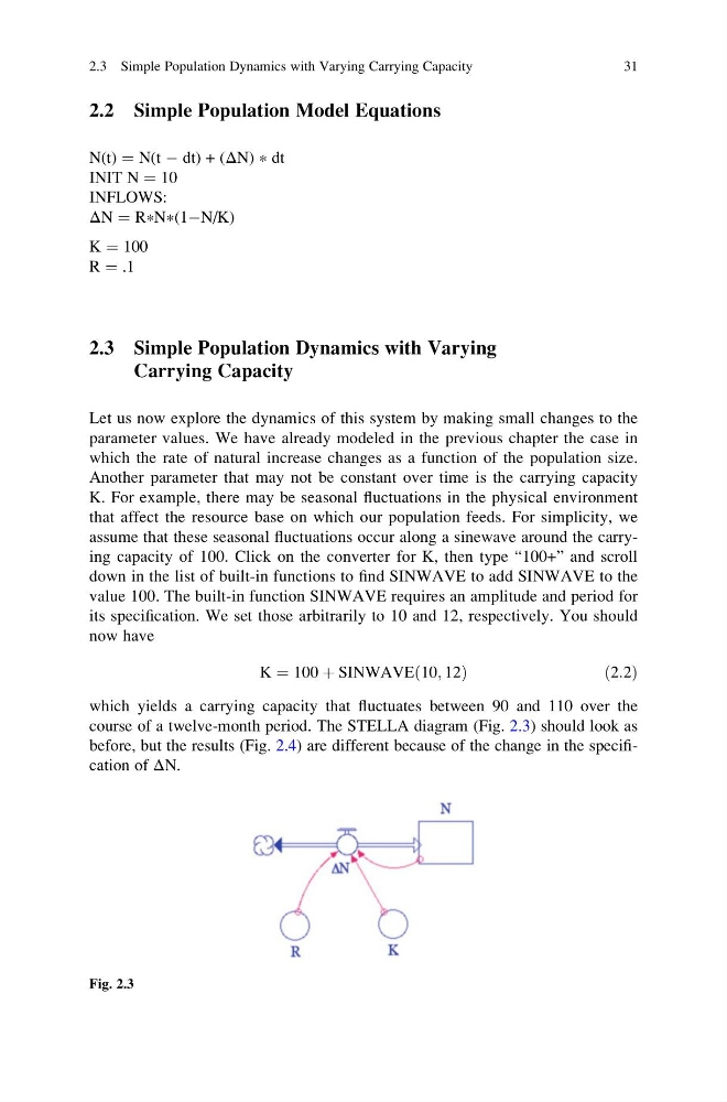
course of a twelve-month period. The STELLA diagram (Fig. 2.3) should look as
before, but the results (Fig. 2.4) are different because of the change in the specification of ΔN.
Fig. 2.3
2.3 Simple Population Dynamics with Varying Carrying Capacity
31
N(t) ¼ N(t À dt) + (ΔN) * dt
INIT N ¼ 10
INFLOWS:
ΔN ¼ R * N * (1ÀN/K)
K ¼ 100
R ¼ .1
2.3 Simple Population Dynamics with Varying
Carrying Capacity
Let us now explore the dynamics of this system by making small changes to the
parameter values. We have already modeled in the previous chapter the case in
which the rate of natural increase changes as a function of the population size.
Another parameter that may not be constant over time is the carrying capacity
K. For example, there may be seasonal fluctuations in the physical environment
that affect the resource base on which our population feeds. For simplicity, we
assume that these seasonal fluctuations occur along a sinewave around the carrying capacity of 100. Click on the converter for K, then type “100+” and scroll
down in the list of built-in functions to find SINWAVE to add SINWAVE to the
value 100. The built-in function SINWAVE requires an amplitude and period for
its specification. We set those arbitrarily to 10 and 12, respectively. You should
now have
K ¼ 100 þ SINWAVE 10; 12
ð
Þ
ð2:2Þ
which yields a carrying capacity that fluctuates between 90 and 110 over the
course of a twelve-month period. The STELLA diagram (Fig. 2.3) should look as
before, but the results (Fig. 2.4) are different because of the change in the specification of ΔN.
Fig. 2.3
2.3 Simple Population Dynamics with Varying Carrying Capacity
31