

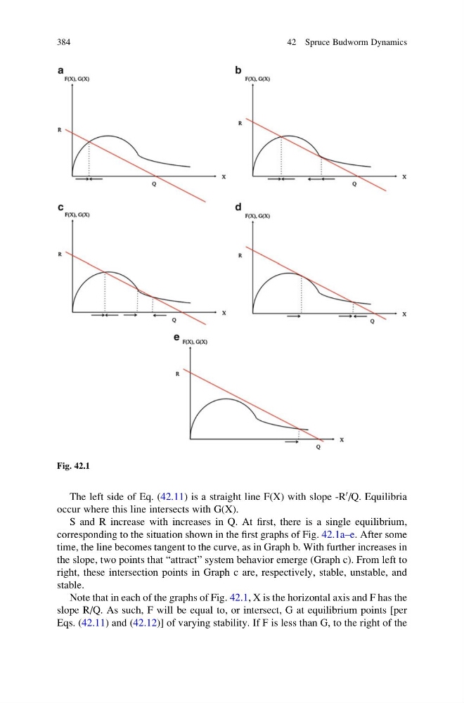
The left side of Eq. (42.11) is a straight line F(X) with slope -R
0 /Q. Equilibria
occur where this line intersects with G(X).
S and R increase with increases in Q. At first, there is a single equilibrium,
corresponding to the situation shown in the first graphs of Fig. 42.1a–e. After some
time, the line becomes tangent to the curve, as in Graph b. With further increases in
the slope, two points that “attract” system behavior emerge (Graph c). From left to
right, these intersection points in Graph c are, respectively, stable, unstable, and
stable.
Note that in each of the graphs of Fig. 42.1, X is the horizontal axis and F has the
slope R/Q. As such, F will be equal to, or intersect, G at equilibrium points [per
Eqs. (42.11) and (42.12)] of varying stability. If F is less than G, to the right of the
Fig. 42.1
384
42 Spruce Budworm Dynamics
0 /Q. Equilibria
occur where this line intersects with G(X).
S and R increase with increases in Q. At first, there is a single equilibrium,
corresponding to the situation shown in the first graphs of Fig. 42.1a–e. After some
time, the line becomes tangent to the curve, as in Graph b. With further increases in
the slope, two points that “attract” system behavior emerge (Graph c). From left to
right, these intersection points in Graph c are, respectively, stable, unstable, and
stable.
Note that in each of the graphs of Fig. 42.1, X is the horizontal axis and F has the
slope R/Q. As such, F will be equal to, or intersect, G at equilibrium points [per
Eqs. (42.11) and (42.12)] of varying stability. If F is less than G, to the right of the
Fig. 42.1
384
42 Spruce Budworm Dynamics