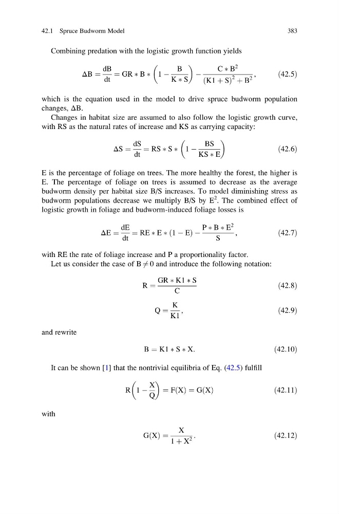
Combining predation with the logistic growth function yields
ΔB ¼
dB
dt
¼ GR Ã B Ã 1 À
B
K Ã S
À
C Ã B
2
K1 þ S
ð
Þ
2 þ B
2
,
ð42:5Þ
which is the equation used in the model to drive spruce budworm population
changes, ΔB.
Changes in habitat size are assumed to also follow the logistic growth curve,
with RS as the natural rates of increase and KS as carrying capacity:
ΔS ¼
dS
dt
¼ RS Ã S Ã 1 À
BS
KS Ã E
ð42:6Þ
E is the percentage of foliage on trees. The more healthy the forest, the higher is
E. The percentage of foliage on trees is assumed to decrease as the average
budworm density per habitat size B/S increases. To model diminishing stress as
budworm populations decrease we multiply B/S by E
2
. The combined effect of
logistic growth in foliage and budworm-induced foliage losses is
ΔE ¼
dE
dt
¼ RE Ã E Ã 1 À E
ð
ÞÀ
P Ã B Ã E
2
S
,
ð42:7Þ
with RE the rate of foliage increase and P a proportionality factor.
Let us consider the case of B 6 ¼ 0 and introduce the following notation:
R ¼
GR Ã K1 Ã S
C
ð42:8Þ
Q ¼
K
K1
,
ð42:9Þ
and rewrite
B ¼ K1 Ã S Ã X:
ð42:10Þ
It can be shown [1] that the nontrivial equilibria of Eq. (42.5) fulfill
R 1 À
X
Q
¼ F X
ð Þ ¼ G X
ð Þ
ð42:11Þ
with
G X
ð Þ ¼
X
1 þ X
2
:
ð42:12Þ
42.1 Spruce Budworm Model
383