

intersection, the point is stable. Thus, between Graph a and Graph d of Fig. 42.1, the
left intersection switches suddenly from stable to unstable, the only stable point
becoming the right intersection. This sudden shift in stable points is the reason
behind the sudden shift, or explosion, in the budworm population. Graph e
in Fig. 42.1 shows the case in which only one point of intersection exists.
This point is a stable attractor.
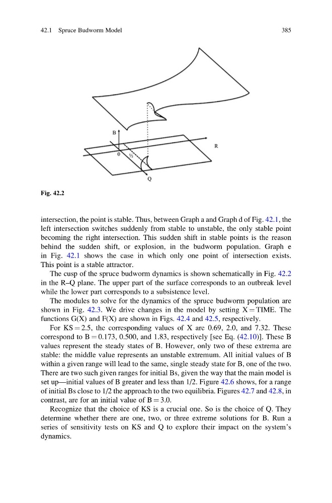
The cusp of the spruce budworm dynamics is shown schematically in Fig. 42.2
in the R–Q plane. The upper part of the surface corresponds to an outbreak level
while the lower part corresponds to a subsistence level.
The modules to solve for the dynamics of the spruce budworm population are
shown in Fig. 42.3. We drive changes in the model by setting X ¼ TIME. The
functions G(X) and F(X) are shown in Figs. 42.4 and 42.5, respectively.
For KS ¼ 2.5, the corresponding values of X are 0.69, 2.0, and 7.32. These
correspond to B ¼ 0.173, 0.500, and 1.83, respectively [see Eq. (42.10)]. These B
values represent the steady states of B. However, only two of these extrema are
stable: the middle value represents an unstable extremum. All initial values of B
within a given range will lead to the same, single steady state for B, one of the two.
There are two such given ranges for initial Bs, given the way that the main model is
set up—initial values of B greater and less than 1/2. Figure 42.6 shows, for a range
of initial Bs close to 1/2 the approach to the two equilibria. Figures 42.7 and 42.8, in
contrast, are for an initial value of B ¼ 3.0.
Recognize that the choice of KS is a crucial one. So is the choice of Q. They
determine whether there are one, two, or three extreme solutions for B. Run a
series of sensitivity tests on KS and Q to explore their impact on the system’s
dynamics.
Fig. 42.2
42.1 Spruce Budworm Model
385
left intersection switches suddenly from stable to unstable, the only stable point
becoming the right intersection. This sudden shift in stable points is the reason
behind the sudden shift, or explosion, in the budworm population. Graph e
in Fig. 42.1 shows the case in which only one point of intersection exists.
This point is a stable attractor.
The cusp of the spruce budworm dynamics is shown schematically in Fig. 42.2
in the R–Q plane. The upper part of the surface corresponds to an outbreak level
while the lower part corresponds to a subsistence level.
The modules to solve for the dynamics of the spruce budworm population are
shown in Fig. 42.3. We drive changes in the model by setting X ¼ TIME. The
functions G(X) and F(X) are shown in Figs. 42.4 and 42.5, respectively.
For KS ¼ 2.5, the corresponding values of X are 0.69, 2.0, and 7.32. These
correspond to B ¼ 0.173, 0.500, and 1.83, respectively [see Eq. (42.10)]. These B
values represent the steady states of B. However, only two of these extrema are
stable: the middle value represents an unstable extremum. All initial values of B
within a given range will lead to the same, single steady state for B, one of the two.
There are two such given ranges for initial Bs, given the way that the main model is
set up—initial values of B greater and less than 1/2. Figure 42.6 shows, for a range
of initial Bs close to 1/2 the approach to the two equilibria. Figures 42.7 and 42.8, in
contrast, are for an initial value of B ¼ 3.0.
Recognize that the choice of KS is a crucial one. So is the choice of Q. They
determine whether there are one, two, or three extreme solutions for B. Run a
series of sensitivity tests on KS and Q to explore their impact on the system’s
dynamics.
Fig. 42.2
42.1 Spruce Budworm Model
385