

DEATH PREY 1 ¼ CONSUME 1
ð40:4Þ
where PREY 1 and PRED 1 are the stock of the two populations in cell 1, BR PREY
1 is the birth rate of prey in cell 1, CONSUME 1 is the number of prey consumed by
predators in cell 1. The number of prey consumed in cell 1 cannot exceed the
number of prey in that cell and is at least zero and at most the consumption rate
times the number of predators in that cell. The amount of prey consumed by
predators in cell 1 is defined as
CONSUME 1 ¼ MIN PREY 1, CONSUME RATE Ã PRED 1
ð
Þ
ð 40:5Þ
CC PREY 1 is the carrying capacity for prey in cell 1. The latter is assumed to
change along a sinewave with an exogenously defined CYCLE TIME:
CC PREY 1 ¼ 2250 Ã SIN 2 Ã PI Ã TIME=CYCLE TIME
ð
Þ þ 2500
ð40:6Þ
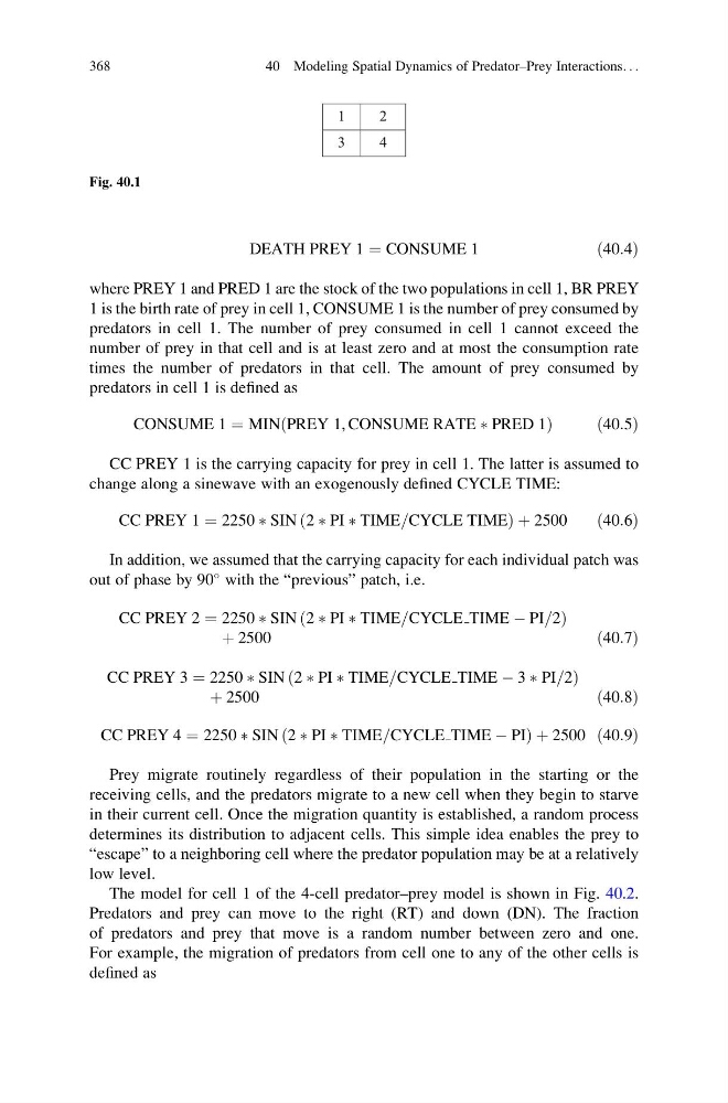
In addition, we assumed that the carrying capacity for each individual patch was
out of phase by 90
with the “previous” patch, i.e.
CC PREY 2 ¼ 2250 Ã SIN 2 Ã PI Ã TIME=CYCLE TIME À PI=2
ð
Þ
þ 2500
ð40:7Þ
CC PREY 3 ¼ 2250 Ã SIN 2 Ã PI Ã TIME=CYCLE TIME À 3 Ã PI=2
ð
Þ
þ 2500
ð40:8Þ
CC PREY 4 ¼ 2250 Ã SIN 2 Ã PI Ã TIME=CYCLE TIME À PI
ð
Þ þ 2500 ð40:9Þ
Prey migrate routinely regardless of their population in the starting or the
receiving cells, and the predators migrate to a new cell when they begin to starve
in their current cell. Once the migration quantity is established, a random process
determines its distribution to adjacent cells. This simple idea enables the prey to
“escape” to a neighboring cell where the predator population may be at a relatively
low level.
The model for cell 1 of the 4-cell predator–prey model is shown in Fig. 40.2.
Predators and prey can move to the right (RT) and down (DN). The fraction
of predators and prey that move is a random number between zero and one.
For example, the migration of predators from cell one to any of the other cells is
defined as
1
2
3
4
Fig. 40.1
368
40 Modeling Spatial Dynamics of Predator–Prey Interactions. . .
ð40:4Þ
where PREY 1 and PRED 1 are the stock of the two populations in cell 1, BR PREY
1 is the birth rate of prey in cell 1, CONSUME 1 is the number of prey consumed by
predators in cell 1. The number of prey consumed in cell 1 cannot exceed the
number of prey in that cell and is at least zero and at most the consumption rate
times the number of predators in that cell. The amount of prey consumed by
predators in cell 1 is defined as
CONSUME 1 ¼ MIN PREY 1, CONSUME RATE Ã PRED 1
ð
Þ
ð 40:5Þ
CC PREY 1 is the carrying capacity for prey in cell 1. The latter is assumed to
change along a sinewave with an exogenously defined CYCLE TIME:
CC PREY 1 ¼ 2250 Ã SIN 2 Ã PI Ã TIME=CYCLE TIME
ð
Þ þ 2500
ð40:6Þ
In addition, we assumed that the carrying capacity for each individual patch was
out of phase by 90
with the “previous” patch, i.e.
CC PREY 2 ¼ 2250 Ã SIN 2 Ã PI Ã TIME=CYCLE TIME À PI=2
ð
Þ
þ 2500
ð40:7Þ
CC PREY 3 ¼ 2250 Ã SIN 2 Ã PI Ã TIME=CYCLE TIME À 3 Ã PI=2
ð
Þ
þ 2500
ð40:8Þ
CC PREY 4 ¼ 2250 Ã SIN 2 Ã PI Ã TIME=CYCLE TIME À PI
ð
Þ þ 2500 ð40:9Þ
Prey migrate routinely regardless of their population in the starting or the
receiving cells, and the predators migrate to a new cell when they begin to starve
in their current cell. Once the migration quantity is established, a random process
determines its distribution to adjacent cells. This simple idea enables the prey to
“escape” to a neighboring cell where the predator population may be at a relatively
low level.
The model for cell 1 of the 4-cell predator–prey model is shown in Fig. 40.2.
Predators and prey can move to the right (RT) and down (DN). The fraction
of predators and prey that move is a random number between zero and one.
For example, the migration of predators from cell one to any of the other cells is
defined as
1
2
3
4
Fig. 40.1
368
40 Modeling Spatial Dynamics of Predator–Prey Interactions. . .