

Chapter 40
Modeling Spatial Dynamics of Predator–Prey
Interactions in a Changing Environment
It is a sad fact that several of our most noble birds of prey can no
longer be studied in what were once their native haunts.
(D. A. Bannerman Birds Brit. Isles, 1956)
40.1 Spatial Predator–Prey Model
In the previous chapter we have modeled the spatial dynamics of species that move
across the landscape to take advantage of differences in habitat characteristics. Let
us now model the case of spatial predator–prey interactions in a changing environment. To model the spatial aspect of these interactions, we define four subdivisions
of the landscape as laid out in Fig. 40.1.
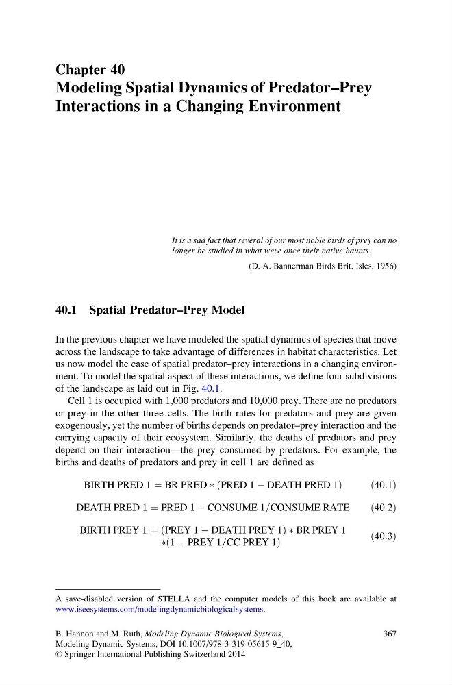
Cell 1 is occupied with 1,000 predators and 10,000 prey. There are no predators
or prey in the other three cells. The birth rates for predators and prey are given
exogenously, yet the number of births depends on predator–prey interaction and the
carrying capacity of their ecosystem. Similarly, the deaths of predators and prey
depend on their interaction—the prey consumed by predators. For example, the
births and deaths of predators and prey in cell 1 are defined as
BIRTH PRED 1 ¼ BR PRED Ã PRED 1 À DEATH PRED 1
ð
Þ
ð 40:1Þ
DEATH PRED 1 ¼ PRED 1 À CONSUME 1=CONSUME RATE
ð40:2Þ
BIRTH PREY 1 ¼ PREY 1 À DEATH PREY 1
ð
Þ Ã BR PREY 1
à 1 À PREY 1=CC PREY 1
ð
Þ
ð40:3Þ
A save-disabled version of STELLA and the computer models of this book are available at
www.iseesystems.com/modelingdynamicbiologicalsystems.
B. Hannon and M. Ruth, Modeling Dynamic Biological Systems,
Modeling Dynamic Systems, DOI 10.1007/978-3-319-05615-9_40,
© Springer International Publishing Switzerland 2014
367
Modeling Spatial Dynamics of Predator–Prey
Interactions in a Changing Environment
It is a sad fact that several of our most noble birds of prey can no
longer be studied in what were once their native haunts.
(D. A. Bannerman Birds Brit. Isles, 1956)
40.1 Spatial Predator–Prey Model
In the previous chapter we have modeled the spatial dynamics of species that move
across the landscape to take advantage of differences in habitat characteristics. Let
us now model the case of spatial predator–prey interactions in a changing environment. To model the spatial aspect of these interactions, we define four subdivisions
of the landscape as laid out in Fig. 40.1.
Cell 1 is occupied with 1,000 predators and 10,000 prey. There are no predators
or prey in the other three cells. The birth rates for predators and prey are given
exogenously, yet the number of births depends on predator–prey interaction and the
carrying capacity of their ecosystem. Similarly, the deaths of predators and prey
depend on their interaction—the prey consumed by predators. For example, the
births and deaths of predators and prey in cell 1 are defined as
BIRTH PRED 1 ¼ BR PRED Ã PRED 1 À DEATH PRED 1
ð
Þ
ð 40:1Þ
DEATH PRED 1 ¼ PRED 1 À CONSUME 1=CONSUME RATE
ð40:2Þ
BIRTH PREY 1 ¼ PREY 1 À DEATH PREY 1
ð
Þ Ã BR PREY 1
à 1 À PREY 1=CC PREY 1
ð
Þ
ð40:3Þ
A save-disabled version of STELLA and the computer models of this book are available at
www.iseesystems.com/modelingdynamicbiologicalsystems.
B. Hannon and M. Ruth, Modeling Dynamic Biological Systems,
Modeling Dynamic Systems, DOI 10.1007/978-3-319-05615-9_40,
© Springer International Publishing Switzerland 2014
367