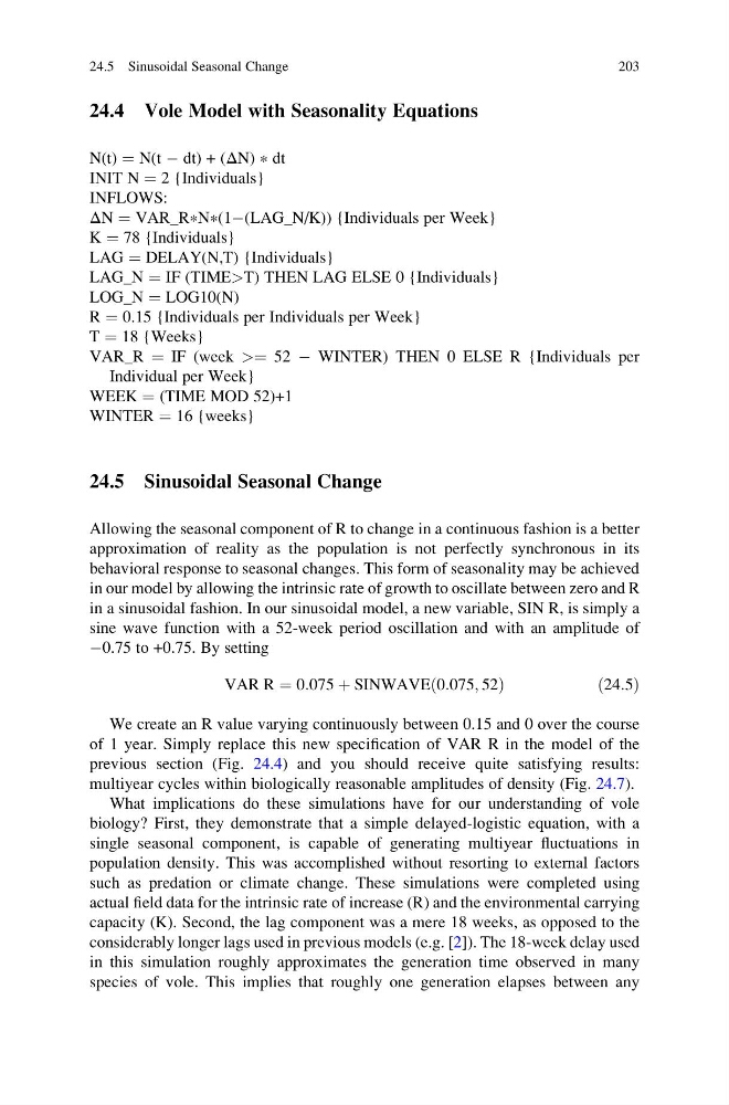
24.4 Vole Model with Seasonality Equations
N(t) ¼ N(t À dt) + (ΔN) * dt
INIT N ¼ 2 {Individuals}
INFLOWS:
ΔN ¼ VAR_R * N * (1À(LAG_N/K)) {Individuals per Week}
K ¼ 78 {Individuals}
LAG ¼ DELAY(N,T) {Individuals}
LAG_N ¼ IF (TIME>T) THEN LAG ELSE 0 {Individuals}
LOG_N ¼ LOG10(N)
R ¼ 0.15 {Individuals per Individuals per Week}
T ¼ 18 {Weeks}
VAR_R ¼ IF (week >¼ 52 À WINTER) THEN 0 ELSE R {Individuals per
Individual per Week}
WEEK ¼ (TIME MOD 52)+1
WINTER ¼ 16 {weeks}
24.5 Sinusoidal Seasonal Change
Allowing the seasonal component of R to change in a continuous fashion is a better
approximation of reality as the population is not perfectly synchronous in its
behavioral response to seasonal changes. This form of seasonality may be achieved
in our model by allowing the intrinsic rate of growth to oscillate between zero and R
in a sinusoidal fashion. In our sinusoidal model, a new variable, SIN R, is simply a
sine wave function with a 52-week period oscillation and with an amplitude of
À0.75 to +0.75. By setting
VAR R ¼ 0:075 þ SINWAVE 0:075; 52
ð
Þ
ð 24:5Þ
We create an R value varying continuously between 0.15 and 0 over the course
of 1 year. Simply replace this new specification of VAR R in the model of the
previous section (Fig. 24.4) and you should receive quite satisfying results:
multiyear cycles within biologically reasonable amplitudes of density (Fig. 24.7).
What implications do these simulations have for our understanding of vole
biology? First, they demonstrate that a simple delayed-logistic equation, with a
single seasonal component, is capable of generating multiyear fluctuations in
population density. This was accomplished without resorting to external factors
such as predation or climate change. These simulations were completed using
actual field data for the intrinsic rate of increase (R) and the environmental carrying
capacity (K). Second, the lag component was a mere 18 weeks, as opposed to the
considerably longer lags used in previous models (e.g. [2]). The 18-week delay used
in this simulation roughly approximates the generation time observed in many
species of vole. This implies that roughly one generation elapses between any
24.5 Sinusoidal Seasonal Change
203