

value for the rest of the year. Run the model and observe the results on a logarithmic
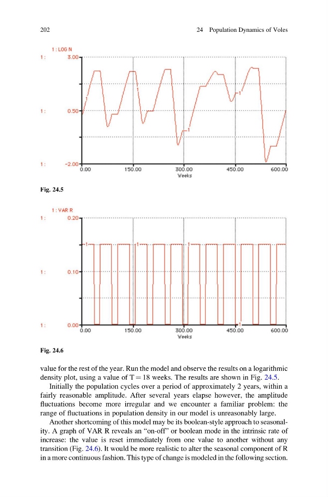
density plot, using a value of T ¼ 18 weeks. The results are shown in Fig. 24.5.
Initially the population cycles over a period of approximately 2 years, within a
fairly reasonable amplitude. After several years elapse however, the amplitude
fluctuations become more irregular and we encounter a familiar problem: the
range of fluctuations in population density in our model is unreasonably large.
Another shortcoming of this model may be its boolean-style approach to seasonality. A graph of VAR R reveals an “on-off” or boolean mode in the intrinsic rate of
increase: the value is reset immediately from one value to another without any
transition (Fig. 24.6). It would be more realistic to alter the seasonal component of R
in a more continuous fashion. This type of change is modeled in the following section.
Fig. 24.5
Fig. 24.6
202
24 Population Dynamics of Voles
density plot, using a value of T ¼ 18 weeks. The results are shown in Fig. 24.5.
Initially the population cycles over a period of approximately 2 years, within a
fairly reasonable amplitude. After several years elapse however, the amplitude
fluctuations become more irregular and we encounter a familiar problem: the
range of fluctuations in population density in our model is unreasonably large.
Another shortcoming of this model may be its boolean-style approach to seasonality. A graph of VAR R reveals an “on-off” or boolean mode in the intrinsic rate of
increase: the value is reset immediately from one value to another without any
transition (Fig. 24.6). It would be more realistic to alter the seasonal component of R
in a more continuous fashion. This type of change is modeled in the following section.
Fig. 24.5
Fig. 24.6
202
24 Population Dynamics of Voles