

LOG_N ¼ LOG10(N) {individuals}
R ¼ .15 {Individuals per Individuals per Week}
T ¼ 12 {weeks}
24.3 Vole Population Dynamics with Seasonality
One shortcoming of our previous model may be its failure to account for seasonal
shifts in behavior. Seasonal changes in the demographics of voles have been well
documented. Let us add seasonality to our delayed-logistic model by varying R, the
intrinsic rate of increase, as a function of time. This modification has a solid
foundation in field data as these rodents are seasonally reproductive; breeding is
sharply curtailed during the winter months. If we assume that limited winter
reproduction is roughly equal to winter mortality, we can allow R to alternate
between zero and its maximum value during the breeding season.
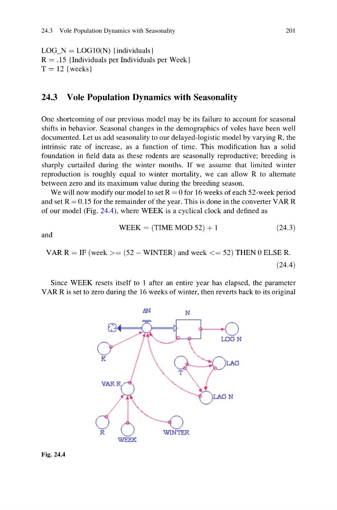
We will now modify our model to set R ¼ 0 for 16 weeks of each 52-week period
and set R ¼ 0.15 for the remainder of the year. This is done in the converter VAR R
of our model (Fig. 24.4), where WEEK is a cyclical clock and defined as
WEEK ¼ TIME MOD 52
ð
Þ þ 1
ð24:3Þ
and
VAR R ¼ IF week >¼ 52 À WINTER
ð
Þ and week <¼ 52
ð
Þ THEN 0 ELSE R:
ð24:4Þ
Since WEEK resets itself to 1 after an entire year has elapsed, the parameter
VAR R is set to zero during the 16 weeks of winter, then reverts back to its original
Fig. 24.4
24.3 Vole Population Dynamics with Seasonality
201
R ¼ .15 {Individuals per Individuals per Week}
T ¼ 12 {weeks}
24.3 Vole Population Dynamics with Seasonality
One shortcoming of our previous model may be its failure to account for seasonal
shifts in behavior. Seasonal changes in the demographics of voles have been well
documented. Let us add seasonality to our delayed-logistic model by varying R, the
intrinsic rate of increase, as a function of time. This modification has a solid
foundation in field data as these rodents are seasonally reproductive; breeding is
sharply curtailed during the winter months. If we assume that limited winter
reproduction is roughly equal to winter mortality, we can allow R to alternate
between zero and its maximum value during the breeding season.
We will now modify our model to set R ¼ 0 for 16 weeks of each 52-week period
and set R ¼ 0.15 for the remainder of the year. This is done in the converter VAR R
of our model (Fig. 24.4), where WEEK is a cyclical clock and defined as
WEEK ¼ TIME MOD 52
ð
Þ þ 1
ð24:3Þ
and
VAR R ¼ IF week >¼ 52 À WINTER
ð
Þ and week <¼ 52
ð
Þ THEN 0 ELSE R:
ð24:4Þ
Since WEEK resets itself to 1 after an entire year has elapsed, the parameter
VAR R is set to zero during the 16 weeks of winter, then reverts back to its original
Fig. 24.4
24.3 Vole Population Dynamics with Seasonality
201