

eventually crash to extinction. Very small time lags reduce the period and amplitude of the oscillation; T < 4 weeks produces only temporary cycles that ultimately
dampen out on the environmental carrying capacity, K. Conversely, increasing T
above 12 increases both the amplitude and period of our cycle.
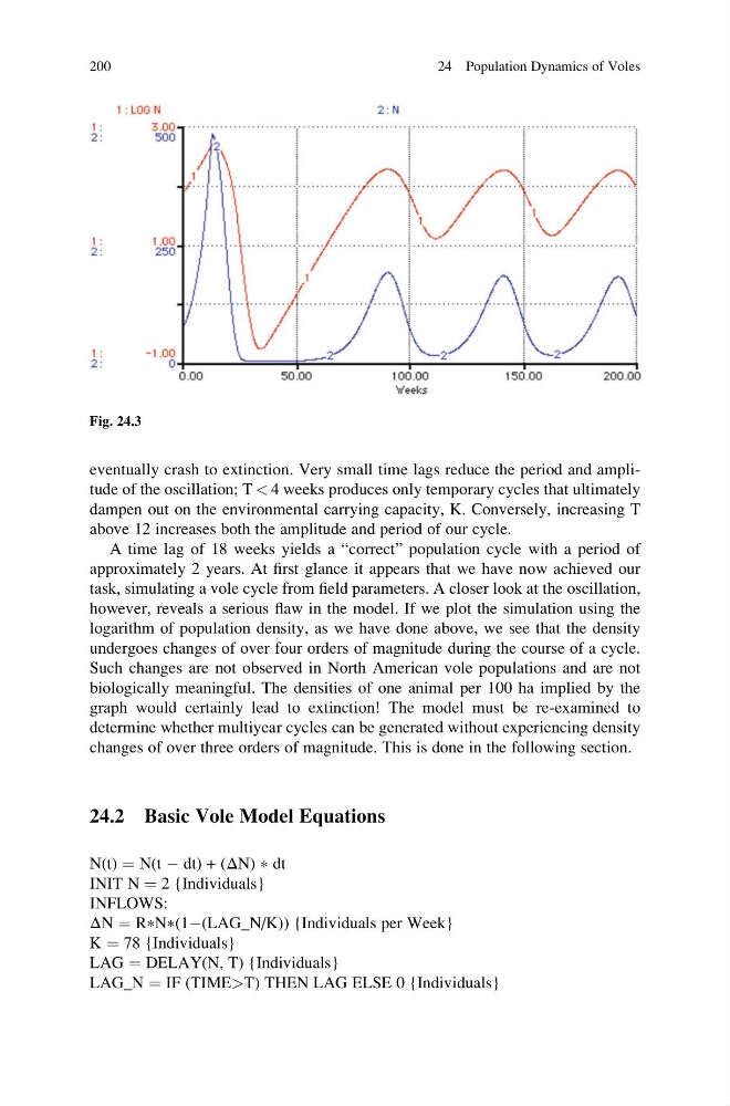
A time lag of 18 weeks yields a “correct” population cycle with a period of
approximately 2 years. At first glance it appears that we have now achieved our
task, simulating a vole cycle from field parameters. A closer look at the oscillation,
however, reveals a serious flaw in the model. If we plot the simulation using the
logarithm of population density, as we have done above, we see that the density
undergoes changes of over four orders of magnitude during the course of a cycle.
Such changes are not observed in North American vole populations and are not
biologically meaningful. The densities of one animal per 100 ha implied by the
graph would certainly lead to extinction! The model must be re-examined to
determine whether multiyear cycles can be generated without experiencing density
changes of over three orders of magnitude. This is done in the following section.
24.2 Basic Vole Model Equations
N(t) ¼ N(t À dt) + (ΔN) * dt
INIT N ¼ 2 {Individuals}
INFLOWS:
ΔN ¼ R * N * (1À(LAG_N/K)) {Individuals per Week}
K ¼ 78 {Individuals}
LAG ¼ DELAY(N, T) {Individuals}
LAG_N ¼ IF (TIME>T) THEN LAG ELSE 0 {Individuals}
Fig. 24.3
200
24 Population Dynamics of Voles
dampen out on the environmental carrying capacity, K. Conversely, increasing T
above 12 increases both the amplitude and period of our cycle.
A time lag of 18 weeks yields a “correct” population cycle with a period of
approximately 2 years. At first glance it appears that we have now achieved our
task, simulating a vole cycle from field parameters. A closer look at the oscillation,
however, reveals a serious flaw in the model. If we plot the simulation using the
logarithm of population density, as we have done above, we see that the density
undergoes changes of over four orders of magnitude during the course of a cycle.
Such changes are not observed in North American vole populations and are not
biologically meaningful. The densities of one animal per 100 ha implied by the
graph would certainly lead to extinction! The model must be re-examined to
determine whether multiyear cycles can be generated without experiencing density
changes of over three orders of magnitude. This is done in the following section.
24.2 Basic Vole Model Equations
N(t) ¼ N(t À dt) + (ΔN) * dt
INIT N ¼ 2 {Individuals}
INFLOWS:
ΔN ¼ R * N * (1À(LAG_N/K)) {Individuals per Week}
K ¼ 78 {Individuals}
LAG ¼ DELAY(N, T) {Individuals}
LAG_N ¼ IF (TIME>T) THEN LAG ELSE 0 {Individuals}
Fig. 24.3
200
24 Population Dynamics of Voles