

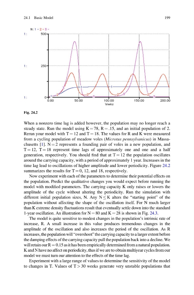
When a nonzero time lag is added however, the population may no longer reach a
steady state. Run the model using K ¼ 78, R ¼ .15, and an initial population of 2.
Rerun your model with T ¼ 12 and T ¼ 18. The values for R and K were measured
from a cycling population of meadow voles (Microtus pennsylvanicus) in Massachusetts [1]. N ¼ 2 represents a founding pair of voles in a new population, and
T ¼ 12, T ¼ 18 represent time lags of approximately one and one and a half
generation, respectively. You should find that at T ¼ 12 the population oscillates
around the carrying capacity, with a period of approximately 1 year. Increases in the
time lag lead to oscillations of higher amplitude and lower periodicity. Figure 24.2
summarizes the results for T ¼ 0, 12, and 18, respectively.
Now experiment with each of the parameters to determine their potential effects on
the population. Predict the qualitative changes you would expect before running the
model with modified parameters. The carrying capacity K only raises or lowers the
amplitude of the cycle without altering the periodicity. Run the simulation with
different initial population sizes, N. Any N K alters the “starting point” of the
population without affecting the shape of the oscillation itself. For N much larger
than K extreme density fluctuations result that eventually settle down into the standard
1-year oscillation. An illustration for N ¼ 80 and K ¼ 28 is shown in Fig. 24.3.
The model is quite sensitive to modest changes in the population’s intrinsic rate of
increase, R. A small increase in this value produces tremendous changes in the
amplitude of the oscillation and also increases the period of the oscillation. As R
increases, the population will “overshoot” the carrying capacity to a larger extent before
the damping effects of the carrying capacity pull the population back into a decline. We
will retain our R ¼ 0.15 as it has been empirically determined from a natural population.
K and N have no affect on periodicity, thus if we are to obtain multiyear cycles from our
model we must turn our attention to the effects of the time lag.
Experiment with a large range of values to determine the sensitivity of the model
to changes in T. Values of T > 30 weeks generate very unstable populations that
Fig. 24.2
24.1 Basic Model
199
steady state. Run the model using K ¼ 78, R ¼ .15, and an initial population of 2.
Rerun your model with T ¼ 12 and T ¼ 18. The values for R and K were measured
from a cycling population of meadow voles (Microtus pennsylvanicus) in Massachusetts [1]. N ¼ 2 represents a founding pair of voles in a new population, and
T ¼ 12, T ¼ 18 represent time lags of approximately one and one and a half
generation, respectively. You should find that at T ¼ 12 the population oscillates
around the carrying capacity, with a period of approximately 1 year. Increases in the
time lag lead to oscillations of higher amplitude and lower periodicity. Figure 24.2
summarizes the results for T ¼ 0, 12, and 18, respectively.
Now experiment with each of the parameters to determine their potential effects on
the population. Predict the qualitative changes you would expect before running the
model with modified parameters. The carrying capacity K only raises or lowers the
amplitude of the cycle without altering the periodicity. Run the simulation with
different initial population sizes, N. Any N K alters the “starting point” of the
population without affecting the shape of the oscillation itself. For N much larger
than K extreme density fluctuations result that eventually settle down into the standard
1-year oscillation. An illustration for N ¼ 80 and K ¼ 28 is shown in Fig. 24.3.
The model is quite sensitive to modest changes in the population’s intrinsic rate of
increase, R. A small increase in this value produces tremendous changes in the
amplitude of the oscillation and also increases the period of the oscillation. As R
increases, the population will “overshoot” the carrying capacity to a larger extent before
the damping effects of the carrying capacity pull the population back into a decline. We
will retain our R ¼ 0.15 as it has been empirically determined from a natural population.
K and N have no affect on periodicity, thus if we are to obtain multiyear cycles from our
model we must turn our attention to the effects of the time lag.
Experiment with a large range of values to determine the sensitivity of the model
to changes in T. Values of T > 30 weeks generate very unstable populations that
Fig. 24.2
24.1 Basic Model
199